Analytical analysis on damping characteristics of rotor system

Wu, Min; Yang, Shengbo; Bao, Wen; Yang, Jinfu

doi:10.21595/jve.2017.18133

Journal of Vibroengineering

Browse Journal

Submit article

Published: 15 May 2017

Check for updates

Analytical analysis on damping characteristics of rotor system

Min Wu¹

Shengbo Yang²

Wen Bao³

Jinfu Yang⁴

^{1, 2, 3}School of Energy Science and Engineering, Harbin Institute of Technology, Harbin, China

⁴Institute of Engineering Thermophysics, Chinese Academy of Sciences, Beijing, China

Corresponding Author:

Min Wu

Cite the article Download PDF

Downloads 1427

Abstract

A general vibration model of a flexible rotor system is established to investigate the influences of the damping characteristics on vibration behaviors. Based on the multi-scale method, the analytical solutions of steady-state and transient-state are derived under the positive and negative conditions of nonlinear damping. The physical significance of the coefficients and their influences on rotor behaviors are analyzed through theoretical analysis and numerical calculation. The experimental results elaborate the damping effect and verify the rationality of the model.

1. Introduction

Rotating machinery is widely used in generators, gas turbines, aero engines and other important power systems. It is the key component and core technology in the national defense industry and energy field such as aerospace, ship engineering and distributed energy. In the development towards high efficiency and high performance, due to its complicated structure, precise design and rigorous assembly, a high-speed flexible rotor system often occurs various faults and shows strong nonlinear behavior characteristics in practical operations. Thus, the stability mechanism of nonlinear rotor system becomes vital to meet the higher requirements of theoretical researches and engineering applications.

For a general rotor system, external damping is considered to be able to reduce the amplitude in the entire operating range and increase the system performance against interference. On the contrary, internal damping is considered to increase the amplitude in operating range, cause oil/gas film whirl, whip and other nonlinear phenomena, and even lead to system failure and halt. The internal damping is caused by the tangential force when stress center line and strain center line of rotor cross-section are no longer coincide. If external damping is insufficient to overcome the self-excited vibration caused by internal damping, the rotor system may become instable.

Newkirk [1] first discovered this phenomenon. Kimball [2] considered the instability was caused by internal friction. Timoshenko [3] did the quantitative analysis and derived the constitutive relation between stress and strain. Gunter [4] and Ehrich [5] also studied the effects of internal friction/damping on the stability of the rotor system respectively. Due to the limitations of linear theory in the analysis of nonlinear phenomena, the accuracy of linearization cannot meet the engineering requirements, so the theory of oil film instability develops from the eigenvalue criterion stability theory based on linear assumption, to the nonlinear stability theory based on nonlinear simulation such as energy method, spectrum analysis method, pumping method [6] and circumferential average velocity ratio method [7]. Tasker [8] used moving-block technique and the sparse time domain method to estimate the equivalent nonlinear damping from transient response data. Chandra [9] used the envelope of free vibration signal extracted by continuous wavelet transform approach to identify nonlinear external and internal damping, and the approximate analytical solution was obtained by Krylov-Bogobliubov method. The nonlinear dynamic stability research has received more and more attention [10].

In this paper, by introducing nonlinear damping force and nonlinear stiffness force, a general form of nonlinear vibration model is proposed for a high-speed flexible rotor system. The steady-state solution and transient-state solution are deduced respectively under positive and negative nonlinear damping conditions via multi-scale method. The effects of linear and nonlinear damping on rotor vibration characteristics are discussed through analytical analysis and numerical simulation, and are elaborated through experimental results.

2. General model establishment

Consider a general ideal single-span single-disc rotor of disc mass $m$ , eccentricity $r$ , rotational frequency $Ω$ , as shown in Fig. 1. Shaft mass is ignored, and counterclockwise is positive. Though the rotor structure is simple, it can fully reflect the linear and nonlinear dynamic behaviors of the rotor system.

Fig. 1Schematic of force analysis of a rotor system

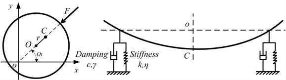
For general liquid or gas bearing, in this paper consider only the bearing support force, ignoring the tangential force. Based on Newton’s second law, equation of motion in the $x$ -axis direction can be described as:

1

m {\ddot{x}}_{c} = F (x, \dot{x}),

where:

2

x_{C} = x + r c o s Ω t .

Generally, the rotor force can be divided into stiffness and damping force by the physical properties, and also can be divided into linear and nonlinear force by mathematical properties, namely:

3

\begin{array}{l} F (x, \dot{x}) = f_{k} (x) + f_{c} (\dot{x}), \\ F (x, \dot{x}) = ξ f_{l} + ε f_{n} = ξ (f_{l} + Θ f_{n}), \end{array}

where $f_{k}$ is elastic force, $f_{c}$ is damping force, $f_{l}$ is linear force, $f_{n}$ is nonlinear force, $ξ$ is linear scale factor, $ε$ is nonlinear scale factor, $Θ = ε / ξ$ is mix ratio. The nonlinear terms have been discussed in detail in previous work [11, 12]. Considering the nonlinear Hooke’s law [13-15] and nonlinear damping force [16, 17], the $f_{k}$ and $f_{c}$ are given as:

4

f_{k} (x) = - \frac{d U}{d x} = - \sum_{n = 0}^{m} k_{n} x^{2 n + 1}, f_{c} (\dot{x}) = - \sum_{n = 1}^{m} c_{n} {|\dot{x}|}^{n - 1} \dot{x} .

In the formulae above, the first order approximation are the traditional linear force expressions $f_{k} = - k x$ and $f_{c} = - c \dot{x}$ . If $n = 0$ for $f_{c}$ , then $f_{c}$ becomes dry friction which is irrelevant to velocity, so it is not considered. In this paper, the nonlinear forces are taken as the first two orders approximation:

5

f_{k} (x) = - k x - η x^{3} = - ξ_{k} (x + Θ_{k} x^{3}), f_{c} (\dot{x}) = - c \dot{x} \mp γ {\dot{x}}^{2} = - ξ_{c} (\dot{x} \pm Θ_{c} {\dot{x}}^{2}),

where $k$ is linear stiffness coefficient, $η$ is nonlinear stiffness coefficient, $c$ is linear damping coefficient, $γ$ is nonlinear damping coefficient, $ξ_{k} = k$ is stiffness linear scale factor, $ξ_{c} = c$ is damping linear scale factor, $Θ_{k} = η / k$ is stiffness mix ratio, $Θ_{c} = γ / c$ is damping mix ratio, the positive sign before $Θ_{c}$ is for positive nonlinear damping and negative sign for negative nonlinear damping. By taken Eq. (2), Eq. (3) and Eq. (5) into Eq. (1), the general form of nonlinear vibration model for a rotor system can be obtained:

6

m \ddot{x} + ξ_{c} (\dot{x} \pm Θ_{c} {\dot{x}}^{2}) + ξ_{k} (x + Θ_{k} x^{3}) = m Ω^{2} r c o s Ω t .

For briefness and clarity, some substitutions are given as:

7

\begin{array}{l} ω_{0}^{2} = \frac{k}{m}, & ε β_{0}^{2} = \frac{η}{m}, & μ = \frac{c}{2 m}, & ε α_{0}^{2} = \frac{γ}{m} \end{array},

where $ω_{0}$ is natural frequency, $β_{0}$ is nonlinear stiffness amplification coefficient, $μ$ is nondimensional linear damping coefficient, $α_{0}$ is nonlinear damping amplification coefficient. Thus $ξ_{k} = ω_{0}^{2} m$ , $Θ_{k} = ε β_{0}^{2} / ω_{0}^{2}$ , $ξ_{c} =$ 2 μm, $Θ_{c} = ε α_{0}^{2} / 2 μ$ , and there are:

8

\ddot{x} + 2 μ \dot{x} \pm ε α_{0}^{2} {\dot{x}}^{2} + ω_{0}^{2} x + ε β_{0}^{2} x^{3} = Ω^{2} r c o s Ω t .

The equation is the nonlinear vibration model based on large deformation and large perturbation assumption for high-speed flexible rotor system. It is worth noting that, the positive sign before velocity square term indicates positive nonlinear damping, and the negative sign indicates negative nonlinear damping.

3. Deduction and analytical solutions

The quadratic approximate solution of Eq. (8) is deduced via multi-scale method:

9

x = x_{0} (T_{0}, T_{1}) + ε x_{1} (T_{0}, T_{1}), T_{0} = t, T_{1} = ε t .

Take Eq. (9) into Eq. (8), according to the power orders of $ε$ , and $D$ is a partial differential operator, there are:

10

ε^{0} : D_{0}^{2} x_{0} + 2 μ D_{0} x_{0} + ω_{0}^{2} x_{0} = \frac{1}{2} Ω^{2} r (e^{j Ω T_{0}} + e^{- j Ω T_{0}}),

11

ε^{1} : D_{0}^{2} x_{1} + 2 μ D_{0} x_{1} + ω_{0}^{2} x_{1} = - 2 D_{0} D_{1} x_{0} - 2 μ D_{1} x_{0} \mp α_{0}^{2} {(D_{0} x_{0})}^{2} - β_{0}^{2} x_{0}^{3} .

The solution of Eq. (10) is:

12

\begin{array}{l} x_{0} = C (T_{1}) e^{r_{1} T_{0}} + \bar{C} (T_{1}) e^{{\bar{r}}_{1} T_{0}} + Q e^{j Ω T_{0}} + \bar{Q} e^{- j Ω T_{0}}, \\ r_{1} = - μ + j \sqrt{ω_{0}^{2} - μ^{2}},^{} Q = \frac{1}{2} \frac{Ω^{2} r}{ω_{0}^{2} - Ω^{2} + 2 j μ Ω}, \end{array}

where $C$ is an unknown complex function, the overline represents the conjugate function. Take Eq. (12) into Eq. (11):

13

\begin{array}{l} D_{0}^{2} x_{1} + 2 μ D_{0} x_{1} + ω_{0}^{2} x_{1} = - [2 D_{1} C (r_{1} + μ) + 6 β_{0}^{2} C Q \bar{Q} + 3 β_{0}^{2} C^{2} \bar{C} e^{- 2 μ T_{0}}] e^{r_{1} T_{0}} \\ \mp α_{0}^{2} Q \bar{Q} Ω^{2} \mp α_{0}^{2} C \bar{C} r_{1} {\bar{r}}_{1} e^{- 2 μ T_{0}} - 3 β_{0}^{2} Q^{2} \bar{Q} e^{j Ω T_{0}} \pm α_{0}^{2} Q^{2} Ω^{2} e^{2 j Ω T_{0}} - β_{0}^{2} Q^{3} e^{3 j Ω T_{0}} \\ \mp 2 j α_{0}^{2} C r_{1} Q Ω e^{r_{1} T_{0} + j Ω T_{0}} \pm 2 j α_{0}^{2} C r_{1} \bar{Q} Ω e^{r_{1} T_{0} - j Ω T_{0}} - 6 β_{0}^{2} C \bar{C} Q e^{- 2 μ T_{0} + j Ω T_{0}} \\ ^{} - 3 β_{0}^{2} C^{2} Q e^{2 r_{1} T_{0} + j Ω T_{0}} - 3 β_{0}^{2} C^{2} \bar{Q} e^{2 r_{1} T_{0} - j Ω T_{0}} - 3 β_{0}^{2} C Q^{2} e^{r_{1} T_{0} + 2 j Ω T_{0}} \\ - 3 β_{0}^{2} C {\bar{Q}}^{2} e^{r_{1} T_{0} - 2 j Ω T_{0}} \mp α_{0}^{2} C^{2} r_{1}^{2} e^{2 r_{1} T_{0}} - β_{0}^{2} C^{3} e^{3 r_{1} T_{0}} + c c, \end{array}

where $c c$ represents the conjugate functions of each term at the right side of the equal sign. The coefficient of first term $e^{r_{1} T_{0}}$ must be zero to avoid duration term. At any point without acceleration, $T_{0} = 0$ , so $e^{- 2 μ T_{0}} = 1$ . There is:

14

2 D_{1} C (r_{1} + μ) + 6 β_{0}^{2} C Q \bar{Q} + 3 β_{0}^{2} C^{2} \bar{C} = 0 .

Assuming $C = a e^{j φ} / 2$ , $C$ can be obtained:

15

C = \frac{1}{2} a_{0} \exp (j \frac{\frac{6 β_{0}^{2} Ω^{4} r^{2}}{{(ω_{0}^{2} - Ω^{2})}^{2} + 4 μ^{2} Ω^{2}} + 3 β_{0}^{2} a_{0}^{2}}{8 \sqrt{ω_{0}^{2} - μ^{2}}} T_{1} + j φ_{0}),

where $a_{0}$ , $φ_{0}$ are the integration constants which can be determined by initial conditions. Take Eq. (15) into Eq. (13) so $x_{1}$ can be solved, then the solution $x$ is:

16

\begin{array}{l} x = A_{0} c o s (Ω t + θ_{0}) + A_{1} c o s (Ω t + θ_{1}) \pm A_{2} c o s (2 Ω t + θ_{2}) + A_{3} c o s (3 Ω t + θ_{3}) \pm A_{4} \\ ^{} + a_{0} e^{- μ t} c o s (ω t + φ_{0}) + A_{01} e^{- 2 μ t} c o s Ω t \pm A_{40} e^{- 2 μ t} \\ ^{} \pm A_{11} e^{- μ t} c o s ((ω + Ω) t + θ_{11}) \pm A_{11^{'}} e^{- μ t} c o s ((ω - Ω) t + θ_{11^{'}}) \\ ^{} + A_{21} e^{- 2 μ t} c o s ((2 ω + Ω) t + θ_{21}) + A_{21^{'}} e^{- 2 μ t} c o s ((2 ω - Ω) t + θ_{21^{'}}) \\ ^{} + A_{12} e^{- μ t} c o s ((ω + 2 Ω) t + θ_{12}) + A_{12^{'}} e^{- μ t} c o s ((ω - 2 Ω) t + θ_{12^{'}}) \\ ^{} \pm A_{20} e^{- 2 μ t} c o s (2 ω t + θ_{20}) + A_{30} e^{- 3 μ t} c o s (3 ω t + θ_{30}), \end{array}

where:

17

λ = \frac{ω_{0}}{Ω}, δ = \frac{2 μ}{Ω}, ω = \frac{1}{2} Ω \sqrt{4 λ^{2} - δ^{2}} + \frac{3 ε β_{0}^{2} (2 A_{0}^{2} + a_{0}^{2})}{4 Ω \sqrt{4 λ^{2} - δ^{2}}}, A_{0} = \frac{r}{\sqrt{{(λ^{2} - 1)}^{2} + δ^{2}}},

A_{1} = - \frac{3 ε β_{0}^{2}}{4 Ω^{2} r} A_{0}^{4}, A_{2} = \frac{ε α_{0}^{2}}{2 \sqrt{{(λ^{2} - 4)}^{2} + 4 δ^{2}}} A_{0}^{2}, A_{3} = - \frac{ε β_{0}^{2}}{4 Ω^{2} \sqrt{{(λ^{2} - 9)}^{2} + 9 δ^{2}}} A_{0}^{3},

A_{4} = - \frac{ε α_{0}^{2}}{2 λ^{2}} A_{0}^{2}, A_{01} = - \frac{3 ε β_{0}^{2} a_{0}^{2}}{2 Ω^{2} r} A_{0}^{2}, A_{40} = - \frac{1}{2} ε α_{0}^{2} a_{0}^{2},

A_{11} = - \frac{ε α_{0}^{2} a_{0} λ}{\sqrt{4 λ^{2} - δ^{2}} + 1} A_{0}, A_{11^{'}} = - \frac{ε α_{0}^{2} a_{0} λ}{\sqrt{4 λ^{2} - δ^{2}} - 1} A_{0},

A_{21} = \frac{3 ε β_{0}^{2} a_{0}^{2}}{4 Ω^{2} \sqrt{{(3 λ^{2} + 1 - δ^{2} + 2 \sqrt{4 λ^{2} - δ^{2}})}^{2} + {(δ \sqrt{4 λ^{2} - δ^{2}} + δ)}^{2}}} A_{0},

A_{21^{'}} = \frac{3 ε β_{0}^{2} a_{0}^{2}}{4 Ω^{2} \sqrt{{(3 λ^{2} + 1 - δ^{2} - 2 \sqrt{4 λ^{2} - δ^{2}})}^{2} + {(δ \sqrt{4 λ^{2} - δ^{2}} - δ)}^{2}}} A_{0},

A_{12} = \frac{3 ε β_{0}^{2} a_{0}}{8 Ω^{2} (\sqrt{4 λ^{2} - δ^{2}} + 2)} A_{0}^{2}, A_{12^{'}} = \frac{3 ε β_{0}^{2} a_{0}}{8 Ω^{2} (- \sqrt{4 λ^{2} - δ^{2}} + 2)} A_{0}^{2},

A_{20} = \frac{ε α_{0}^{2} a_{0}^{2} \sqrt{{(- 2 λ^{2} + δ^{2})}^{2} + δ^{2} (4 λ^{2} - δ^{2})}}{4 \sqrt{{(3 λ^{2} - δ^{2})}^{2} + δ^{2} (4 λ^{2} - δ^{2})}},

A_{30} = \frac{ε β_{0}^{2} a_{0}^{3}}{4 Ω^{2} \sqrt{{(8 λ^{2} - 3 δ^{2})}^{2} + 9 δ^{2} (4 λ^{2} - δ^{2})}}, θ_{0} = - a r c t g \frac{δ}{λ^{2} - 1}, θ_{1} = 2 θ_{0},

θ_{2} = - a r c t g \frac{2 δ}{λ^{2} - 4} + 2 θ_{0}, θ_{3} = - a r c t g \frac{3 δ}{λ^{2} - 9} + 3 θ_{0},

θ_{11} = a r c t g \frac{δ}{\sqrt{4 λ^{2} - δ^{2}}} + θ_{0} + φ_{0}, θ_{11'} = a r c t g \frac{δ}{\sqrt{4 λ^{2} - δ^{2}}} - θ_{0} + φ_{0},

θ_{21} = - a r c t g \frac{δ \sqrt{4 λ^{2} - δ^{2}} + δ}{3 λ^{2} + 1 - δ^{2} + 2 \sqrt{4 λ^{2} - δ^{2}}} + θ_{0} + 2 φ_{0},

θ_{21^{'}} = - a r c t g \frac{δ \sqrt{4 λ^{2} - δ^{2}} - δ}{3 λ^{2} + 1 - δ^{2} - 2 \sqrt{4 λ^{2} - δ^{2}}} - θ_{0} + 2 φ_{0},

θ_{12} = 2 θ_{0} + φ_{0}, θ_{12'} = - 2 θ_{0} + φ_{0},

θ_{20} = - a r c t g \frac{δ \sqrt{4 λ^{2} - δ^{2}}}{- 2 λ^{2} + δ^{2}} - a r c t g \frac{δ \sqrt{4 λ^{2} - δ^{2}}}{3 λ^{2} - δ^{2}} + 2 φ_{0},

θ_{30} = - a r c t g \frac{3 δ \sqrt{4 λ^{2} - δ^{2}}}{8 λ^{2} - 3 δ^{2}} + 3 φ_{0},

where $λ$ is rotational speed ratio, $δ$ is damping rotational speed ratio, $A_{i}$ is amplitude, $θ_{i}$ is phase, $ω$ is forced vibration frequency. Eq. (16) is the general solution response of the nonlinear vibration model, including steady-state solution and transient-state solution. The first five terms $A_{0} c o s (Ω t + θ_{0}) + A_{1} c o s (Ω t + θ_{1}) \pm A_{2} c o s (2 Ω t + θ_{2}) + A_{3} c o s (3 Ω t + θ_{3}) \pm A_{4}$ are steady-state solution, and the remaining terms are transient-state solution because they contain the attenuation term $e^{- μ t}$ . For the ± sign of Eq. (16), the positive sign corresponds to the positive nonlinear damping, and the negative sign corresponds to the negative nonlinear damping.

4. Analytical analysis and numerical calculation

4.1. Analytical analysis

The analysis of Eq. (17) can qualitatively elaborates the influences of the coefficients (such as linear stiffness $k$ , linear damping $μ$ , nonlinear stiffness $β_{0}$ , nonlinear damping $α_{0}$ ) on responses. In Eq. (17), all the amplitudes $A_{i}$ , phases $θ_{i}$ and forced vibration frequency $ω$ contain rotational speed ratio $λ$ and damping rotational speed ratio $δ$ . $λ$ , defined as $λ = ω_{0} / Ω = \sqrt{k / m} / Ω$ , is a function of linear stiffness $k$ . $δ$ , defined as $δ = 2 μ / Ω$ , is a function of linear damping $μ$ . Amplitudes $A_{i}$ contain nonlinear stiffness $β_{0}$ and nonlinear damping $α_{0}$ , while phases $θ_{i}$ do not contain the both, and frequency $ω$ contains only $β_{0}$ . It is indicated that both nonlinear coefficients have an impact on amplitudes but not phases, and only nonlinear stiffness has an impact on forced vibration frequency. The following will be a detailed analysis of coefficients’ effects on each parameter.

1. Phases $θ_{i}$ only contain $λ (k)$ and $δ (μ)$ , that is, phases only depend on linear stiffness $k$ and linear damping $μ$ , irrelevant to nonlinear stiffness $β_{0}$ and nonlinear damping $α_{0}$ . Nonlinear forces do not affect the phases change.

2. Forced vibration frequency $ω$ contains $λ$ , $δ$ and $β_{0}$ . Compared with the natural frequency of free vibration $ω = \sqrt{ω_{0}^{2} - μ^{2}} + 3 ε β_{0}^{2} a_{0}^{2} / 8 \sqrt{ω_{0}^{2} - μ^{2}}$ [11, 12], the natural frequency of forced vibration is:

ω = \frac{1}{2} Ω \sqrt{4 λ^{2} - δ^{2}} + \frac{3 ε β_{0}^{2} (2 A_{0}^{2} + a_{0}^{2})}{4 Ω \sqrt{4 λ^{2} - δ^{2}}} = \sqrt{ω_{0}^{2} - μ^{2}} + \frac{6 ε β_{0}^{2} A_{0}^{2} + 3 ε β_{0}^{2} a_{0}^{2}}{8 \sqrt{ω_{0}^{2} - μ^{2}}},

where the additional term $6 ε β_{0}^{2} A_{0}^{2} / 8 \sqrt{ω_{0}^{2} - μ^{2}}$ is the natural frequency correction term caused by the unbalance mass excitation of forced vibration, and this is the difference with that of free vibration model. It can be seen that, if the system adds external excitation, a corresponding correction term will be added into the natural frequency, such as the unbalanced mass excitation can cause a natural frequency correction term of nonlinear stiffness $β_{0}$ and fundamental frequency amplitude $A_{0}$ . The nonlinear damping $α_{0}$ has no effect on the natural frequency.

3. Amplitudes $A_{i}$ contain $λ$ , $δ$ , $β_{0}$ and $α_{0}$ . It is indicated that linear and nonlinear force will affect amplitudes. The specific effects of linear damping $δ (μ)$ and nonlinear damping $α_{0}$ on the steady-state and transient-state amplitudes are analyzed in detail as follows.

4. For linear damping $δ (μ)$ , the $δ^{2}$ term appears in the denominators of the steady-state amplitudes $A_{0} - A_{4}$ , so the steady-state amplitudes decrease as the absolute value of $δ$ increases; the $δ^{2}$ term appears in the denominators of the transient-state amplitudes and also in the numerator of $A_{20}$ .

If linear damping $δ (μ)$ is positive, the $e^{- μ t}$ is an attenuation term, so the transient-state amplitudes can be ignored for they are one magnitude smaller than that of steady-state. The vibration is dominated by steady-state, and the amplitudes decrease as the absolute value of $δ$ increases. If $δ (μ)$ is negative, the $e^{- μ t}$ becomes a divergence term, so the transient-state amplitudes are much larger than that of steady-state. The vibration is dominated by transient-state, and the amplitudes increase as the absolute value of $δ$ increases. That is, positive $δ$ can restrain vibration, negative $δ$ can intensify vibration, and this is consistent with the phenomenon in engineering practice.

Moreover, this is also consistent with the classical theory that negative damping can lead to system instability, and in this paper a more detailed mechanism analysis is given by using analytical expressions of steady-state and transient-state. If $δ$ is positive, it can restrain both steady-state and transient-state amplitudes, so the positive linear damping can restrain the vibration, which is unquestionable. If $δ$ is negative, though it can still restrain steady-state amplitudes, the restraint effect is much smaller than the divergence effect on transient-state amplitudes, so the total amplitudes increase rapidly and the negative linear damping can cause instability. Of course, this theoretical analysis still needs further experimental verification.

5. For nonlinear damping $α_{0}$ , the $α_{0}^{2}$ term appears only in the numerators of the steady-state amplitudes $A_{2}, A_{4}$ and the transient-state amplitudes $A_{40},$ $A_{11},$ $A_{11^{'}},$ $A_{20},$ so the amplitudes increase as the absolute value of $α_{0}$ increases. Thus, nonlinear damping can intensify vibration. However, the amplitude change caused by nonlinear damping is smaller than that of linear damping. The quantitative comparisons of response curves are in the following Section 4.2.

Apparently, by analyzing the parameter expressions Eq. (17), it can be seen that: (1) Phase modulation is related to linear stiffness $k$ and linear damping $μ$ . (2) Frequency modulation is related to nonlinear stiffness $β_{0}$ , $k$ , $μ$ . (3) Amplitude modulation is related to nonlinear damping $α_{0}$ , $β_{0}$ , $k$ , $μ$ . All the coefficients are constants, and the machanism analysis for damping on steady-state and transient-state solution needs to be further verified by experiments.

4.2. Numerical calculation

The theoretical calculation parameters are as follows: $m =$ 1 kg, $k =$ 1×10⁴ N/m, $μ =$ 12 rad/s, $ω_{0} =$ 100 rad/s, $r =$ 1×10^-5 m, $η = ε β_{0}^{2} m =$ 2.5×10¹² N/m³, $γ = ε α_{0}^{2} m =$ 9×10⁴ Ns²/m². Using MATLAB software, the influence of the coefficients on the amplitudes, phases and responses of the general solution are calculated and analyzed.

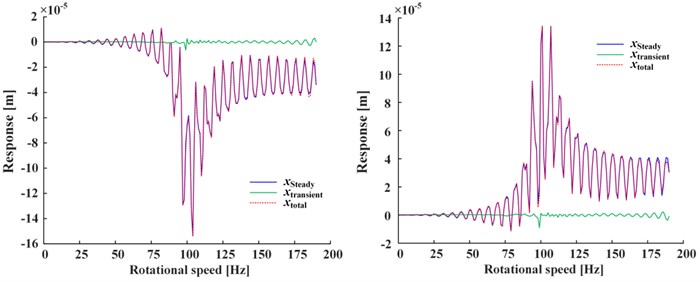
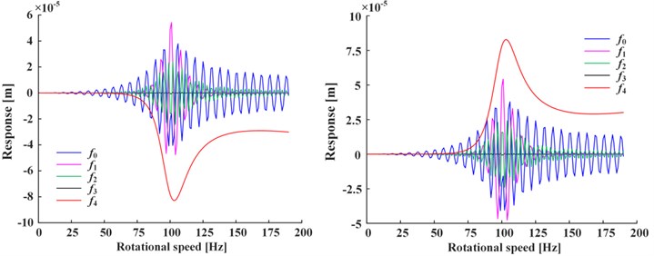
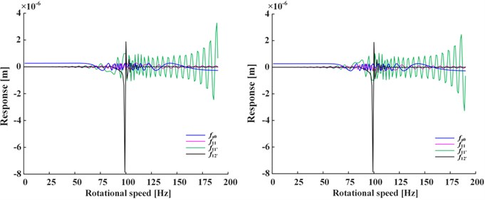
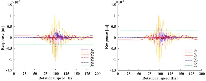
Fig. 2 shows the total response of Fig. 2(a), steady-state response of Fig. 2(b) and transient-state response of Fig. 2(c, d) under the conditions of positive nonlinear damping (left) and negative nonlinear damping (right), where $x_{t o t a l}$ , $x_{s t e a d y}$ , $x_{t r a n s i e n t}$ represent the general solution (i.e., the sum of steady-state and transient-state), steady-state solution and transient-state solution respectively, $f_{i}$ represents the response of corresponding term $A_{i} \times c o s ()$ in which the subscript is the same. For the steady-state response, it is obviously that $f_{3}$ is the smaller one in Fig. 2(b). For the transient-state response, $f_{a 0}$ , $f_{11}$ , $f_{11^{'}}$ , $f_{12^{'}}$ are the larger ones in Fig. 2(c) while the rest smaller ones in Fig. 2(d). The transient-state response is about two orders of magnitude smaller than the steady-state response.

Fig. 2a) The total, b) steady-state and c), d) transient-state response (left: positive nonlinear damping, right: negative nonlinear damping)

a)

b)

c)

d)

Compared the two responses under positive and negative nonlinear damping conditions, it can be seen that the response curves which are almost symmetrical about $x$ -axis also have the difference of positive and negative, while the positive and negative of the displacement responses are only represent the difference in vibration direction, and the trend of curves remains the same.

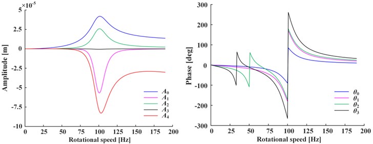
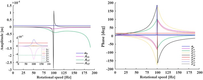
Fig. 3 shows the amplitudes $A_{i}$ and phases $θ_{i}$ of steady-state of Fig. 3(a) and transient-state of Fig. 3(b) under positive nonlinear damping condition. The curves under negative nonlinear damping condition have the same trend, so omitted. As can be seen from the figure, both amplitudes and phases change with rotational speed and have peak value at the critical speed ( $Ω = ω_{0} =$ 100 rad/s), indicating that at critical point the amplitudes will reach extremum and the phases change are the integer multiple of 90 deg. The phases $θ_{2}$ , $θ_{3}$ of steady-state have peak value at 1/2, 1/3 of speed range additionally, which is caused by the second and third harmonic generations.

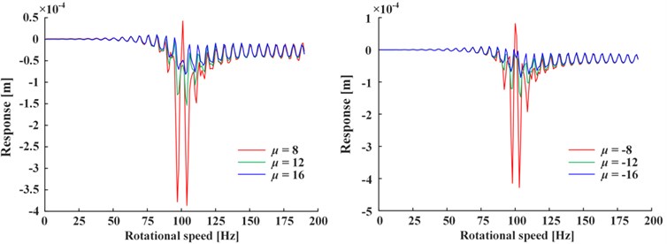
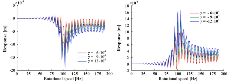
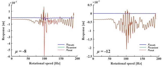
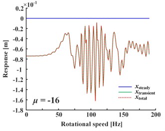
Fig. 4 shows the influence of positive value and negative value change of the linear damping coefficient of Fig. 4(a) and nonlinear damping coefficient of Fig. 4(b) on responses, where the nonlinear damping coefficient is written in the form of $γ = ε α_{0}^{2} m$ for calculation convenience. Note that only negative linear damping coefficient $μ$ corresponds to the steady-state response, while others correspond to the total response (i.e., the sum of steady-state and transient-state). It can be seen from Fig. 4 that the vibration decreases as the absolute value of linear damping increases (only steady-state vibration decreases as $μ$ is negative), and the vibration increases as the absolute value of nonlinear damping increases. If the damping is doubled, the vibration change is less than twice caused by nonlinear damping, and about one order of magnitude caused by linear damping, so nonlinear damping’s impact is less than linear damping’s. If $μ$ is negative, the total response is given in Fig. 5. It is obvious that the magnitude of transient-state response increases rapidly as the attenuation term becomes divergence term, and the steady-state response is negligible.

Fig. 3a) Steady-state and b) transient-state

a)

b)

Fig. 4a) Responses of linear and b) nonlinear damping coefficient (Only negative linear damping’s response is steady-state response, others are total responses.)

a) Responses of linear and b) nonlinear damping coefficient (Only negative linear damping’s response is steady-state response, others are total responses.)

a)

b)

Fig. 5Transient-state response is much larger than steady-state for negative linear damping

Therefore, it can be indicated that: (1) Positive linear damping can restrain vibration. (2) Negative linear damping’s restraint effect on steady-state is far less than the exponential divergence effect on transient-state, so it can intensify vibration. (3) Nonlinear damping can intensify vibration, but its influence is less than that of linear damping.

4.3. Experiment results

Set up a single-disc principle rotor test bed for verification, as shown in Fig. 6. Rotor material with $φ$ 235 steel, disc mass 0.5 kg, disc radius 0.039 m, shaft radius 0.005 m, elastic modulus 200 GPa, Poisson ratio 0.3, bearing span 0.4335 m, disc distance from the left bearing of 0.13005 m. Displacement and phase signals are input to the DASP software for real-time monitoring and analysis [18, 19]. The experiment on the effect of the oil film force of sliding bearing is carried out to verify the damping effect on the vibration behaviors in the nonlinear vibration model proposed in this paper.

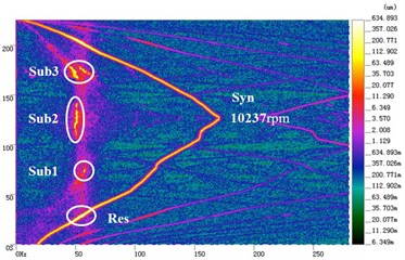
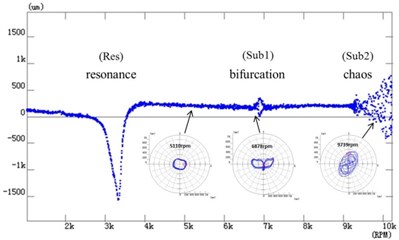
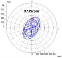
Fig. 7 shows the time-amplitude-frequency spectrum of Fig. 7(a), and the bifurcation diagram of speed-up process of Fig. 7(b). In Fig. 7(a), the rotor is first speed-up then speed-down, the maximum speed of 10237 rpm, where Res is resonance area, Sub1 is oil whirl area, Sub2 is oil whip area and Sub3 is double subharmonic area. In Fig. 7(b), typical shaft orbits are selected for each bifurcation section, namely, period-1 (5110 rpm), bifurcation (6878 rpm) and chaos (9739 rpm), which is shown in detail in Fig. 8.

Fig. 6Single-disc principle rotor test bed

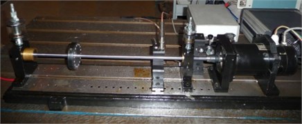
Fig. 7a) Time-amplitude-frequency spectrum and b) bifurcation diagram of speed-up process

a)

b)

Fig. 8Shaft orbits

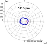
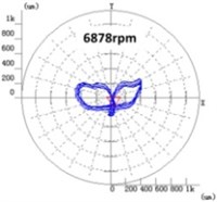
For the vibration behaviors such as rotation and whirl in the experiment, the oil film force model of reference [20] is used to analyze the damping effect, which is also corresponding to the linear damping term $2 μ \dot{x}$ of Eq. (8). The oil film force model [20] is $F_{π} = f_{1} ω_{0} - f_{2} Ω + f_{3} \dot{ε}$ , where $f_{i}$ is positive coefficients, $ω_{0}$ , $Ω$ , $\dot{ε}$ is rotational frequency, whirl frequency and squeezing rate respectively. As can be seen from Fig. 8, the amplitude of shaft orbit increases from period-1 (5110 rpm) to bifurcation (6878 rpm) due to the negative linear damping effect which can reduce the loading capacity of the oil film. It is consistent with the theoretical analysis in this paper.

When the rotational speed is above 9000 rpm, the development path of chaos can be seen clearly from the figure, and the amplitude of shaft orbit increases gradually, such as 9739 rpm. It is because under the combined effects of negative linear damping and nonlinear damping, the subharmonic frequency of self-excited vibration generated by shaft and oil film is close to the natural frequency of the rotor system, which causes the frequency locking resonance, namely the oil film whip phenomenon. When the rotational speed increases in the whip area, the rotational frequency increases, so the positive linear damping increases, which lead to the amplitude decrease; the whirl frequency increases, so the negative linear damping increases, which lead to the amplitude increase. Therefore, the oil film whirl and whip characteristics of the experiment shows that the positive linear damping can restrain vibration, while the negative linear damping and the nonlinear damping can intensify vibration.

5. Conclusions

In this paper, by introducing linear and nonlinear force, a nonlinear vibration model is established for high-speed flexible rotor system, and the analytical solutions are deduced and analyzed. The conclusions are as follows.

1. The general form of nonlinear vibration model is constructed, and the analytical solutions of steady-state and transient-state are derived under the conditions of positive and negative nonlinear damping coefficient.

2. The influence and physical significance of the coefficients on parameters are analyzed. The phase modulation is related to linear stiffness $k$ and linear damping $μ$ . The frequency modulation is related to nonlinear stiffness $β_{0}$ , $k$ , $μ$ . The amplitude modulation is related to nonlinear damping $α_{0}$ , $β_{0}$ , $k$ , $μ$ .

3. Positive linear damping can restrain vibration, while negative linear damping and nonlinear damping can intensify vibration. Nonlinear damping has less influence on vibration than linear damping. The experimental results verify the damping effect and the rationality of the nonlinear vibration model.

References

Newkirk B. L. Shaft whipping. General Electric Review, Vol. 27, 1924, p. 169-178.

Search CrossRef
Kimball A. L. Internal friction as a cause of shaft whirling. Philosophical Magazine, Vol. 49, Issue 292, 1925, p. 724-727.

Publisher
Timoshenko S. Vibration Problem in Engineering. Second Edition, D. van Nostrand Company, New York, 1937.

Search CrossRef
Gunter E. J. The influence of internal friction on the stability of high speed rotors. Journal of Engineering for Industry, Vol. 89, Issue 4, 1967, p. 683-688.

Publisher
Ehrich F. F. Shaft whirl induced by rotor internal damping. Journal of Applied Mechanics, Vol. 31, Issue 2, 1964, p. 279-282.

Publisher
Crandall S. H. Heuristic Explanation of Journal Bearing Instability. Rotordynamic Instability Problems in High-Performance Turbomachinery, NASA CP-2250, 1982.

Search CrossRef
Muszynska A. Whirl and whip-rotor/bearing stability problems. Journal of Sound and Vibration, Vol. 110, Issue 3, 1986, p. 443-462.

Publisher
Tasker F., Chopra I. Nonlinear damping estimation from rotor stability data using time and frequency domain techniques. AIAA Journal, Vol. 30, Issue 5, 1992, p. 1383-1391.

Publisher
ChandraN. H., SekharA. S. Nonlinear damping identification in rotors using wavelet transform. Mechanism and Machine Theory, Vol. 100, 2016, p. 170-183.

Publisher
ZhaoJ., LinnettI., McleanL. Imbalance response and stability of eccentric squeeze-film-damped nonlinear rotor bearing systems. JSME International Journal Series B Fluids and Thermal Engineering, Vol. 37, Issue 4, 1994, p. 886-895.

Publisher
Wu M., Han D., Yang S., et al. Research on nonlinear vibration analytical model of rotor system. Journal of Aerospace Power, 2016, (in Press, in Chinese).

Search CrossRef
Wu M., Yang S., Han D., et al. Analytical model for nonlinear vibration of flexible rotor system. Journal of Vibroengineering, Vol. 18, Issue 8, 2016, p. 4980-4994.

Publisher
Liu B., Peng J. Nonlinear Dynamics. Higher Education Press, Beijing, 2004, (in Chinese).

Search CrossRef
Khalil H. Nonlinear Systems. Electronic Industry Press, Beijing, 2005, (in Chinese).

Search CrossRef
Zhou J., Zhu Y. Nonlinear Vibration. Xi’an Jiaotong University Press, Xi’an, 1998, (in Chinese).

Search CrossRef
Hu H. Nonlinear Vibration. Aviation Industry Press, Beijing, 2000, (in Chinese).

Search CrossRef
Chen Y. Modern Analytical Method in Nonlinear Dynamics. Science Press, Beijing, 1992, (in Chinese).

Search CrossRef
Yang J., Wu M. Single-disc rotor nonlinear vibration model and mechanism. Journal of Aerospace Power, Vol. 27, Issue 8, 2012, p. 1738-1745, (in Chinese).

Search CrossRef
Wu M., Yang J. The research on single-disc rotor nonlinear vibration model and mechanism. Mechatronics and Information Technology, Parts 1 and 2, Vol. 2, Issue 3, 2012, p. 954-959.

Publisher
Yang J., Chen C., Yang S., et al. An analytic model of oil-film force on hydrodynamic journal bearing of finite length. ASME Turbo Expo 2008: Power for Land, Sea and Air, Parts A and B, 2008, p. 947-952.

Publisher

About this article

Received

25 December 2016

Accepted

12 April 2017

Published

15 May 2017

SUBJECTS

Mechanical vibrations and applications

DOI

https://doi.org/10.21595/jve.2017.18133

Keywords

flexible rotor system

general vibration model

analytical solution

nonlinear damping

vibration mechanism

Acknowledgements

The work is supported by National Science and Technology Projects (Grant No. 2012BAA11B02), and the support is gratefully acknowledged.

This is an open access article distributed under the Creative Commons Attribution License, which permits unrestricted use, distribution, and reproduction in any medium, provided the original work is properly cited.

Previous article in issue Previous Next article in issue Next

Research article

2023 10 31

Rigid-flexible coupling modeling of the dual-rotor system for aero-engine

Pingping Ma, Yuehui Dong, Hangqi Zhao, Yang Li, Muge Liu

Research article

2018 08 15

Dynamic response analysis for the aero-engine dual-rotor-bearing system with flexible coupling misalignment faults

Zhenyong Lu, Xiaodong Wang, Lei Hou, Yushu Chen, Hongliang Li

Research article

2018 05 15

Non-probabilistic analysis of a double-disk rotor system with uncertain parameters

Chao Fu, Xingmin Ren, Yongfeng Yang

Research article

2017 03 31

Based on lacing wires influence of coupling vibration of a multi flexible disks turbine rotor system by two methods

Yi-Jui Chiu, Sheng-Rui Jian, Chia-Hao Yang, Guo-Fei Yu

M. Wu, S. Yang, W. Bao, and J. Yang, “Analytical analysis on damping characteristics of rotor system,” Journal of Vibroengineering, Vol. 19, No. 3, pp. 1697–1708, May 2017, https://doi.org/10.21595/jve.2017.18133

Copy Extrica

Copied to clipboard!

TY  - JOUR
DO  - 10.21595/jve.2017.18133
UR  - https://doi.org/10.21595/jve.2017.18133
TI  - Analytical analysis on damping characteristics of rotor system
T2  - Journal of Vibroengineering
AU  - Wu, Min
AU  - Yang, Shengbo
AU  - Bao, Wen
AU  - Yang, Jinfu
PY  - 2017
DA  - 2017/05/15
PB  - JVE International Ltd.
SP  - 1697-1708
IS  - 3
VL  - 19
SN  - 1392-8716
ER  - 

Copy Ris

Copied to clipboard!

@article{Wu_2017,
	doi = {10.21595/jve.2017.18133},
	url = {https://doi.org/10.21595/jve.2017.18133},
	year = 2017,
	month = {may},
	publisher = {{JVE} International Ltd.},
	volume = {19},
	number = {3},
	pages = {1697--1708},
	author = {Min Wu and Shengbo Yang and Wen Bao and Jinfu Yang},
	title = {Analytical analysis on damping characteristics of rotor system},
	journal = {Journal of Vibroengineering}
}

Copy Bibtex

Copied to clipboard!

[1]M. Wu, S. Yang, W. Bao, and J. Yang, “Analytical analysis on damping characteristics of rotor system,” Journal of Vibroengineering, vol. 19, no. 3, pp. 1697–1708, May 2017, doi: 10.21595/jve.2017.18133.

Copy IEEE

Copied to clipboard!

Wu, Min, Shengbo Yang, Wen Bao, and Jinfu Yang. “Analytical Analysis on Damping Characteristics of Rotor System.” Journal of Vibroengineering 19, no. 3 (May 15, 2017): 1697–1708. https://doi.org/10.21595/jve.2017.18133.

Copy Chicago

Copied to clipboard!

Analytical analysis on damping characteristics of rotor system

Abstract

1. Introduction

2. General model establishment

3. Deduction and analytical solutions

4. Analytical analysis and numerical calculation

4.1. Analytical analysis

4.2. Numerical calculation

4.3. Experiment results

5. Conclusions

References

About this article

Related Articles