Engine power measurement without external load based on vibration signal

Zhang, Shuai; Zeng, Ruili

doi:10.21595/jve.2017.18788

Journal of Vibroengineering

Browse Journal

Submit article

Published: 15 November 2017

Check for updates

Engine power measurement without external load based on vibration signal

Shuai Zhang¹

Ruili Zeng²

¹Postgraduate Training Brigade, Army Military Transportation University, Tianjin, China

²Military Vehicle Department, Army Military Transportation University, Tianjin, China

Corresponding Author:

Ruili Zeng

Cite the article Download PDF

Downloads 1407

CrossRef Citations 1

Abstract

The vibration signals from engines contain information about the engine conditions. Engine power is an important parameter that indicates the state of an engine. In this manuscript, a method for measuring the engine power, using the vibration signals from the engine, is developed. In our proposed method, the power of the engine is measured based on the principle of no-load measurement. The discrete values of rotation speed are computed from the vibration signal, using wavelet transforms, the Hilbert envelope, and three autocorrelations. By comparing various curve-fitting and interpolation methods, an optimal method for curve fitting the discrete acceleration data is chosen, and the corresponding times of the starting speed and terminal speed are calculated using the analytical formulas of the fitted curve. Finally, the maximum engine power is obtained from the calibration tests. Experimental results show that the overall performance is good and that the maximum power measurement accuracy is 98.4 % after accurate calibration. This meets the requirements of the power measurement accuracy under the condition of no load.

1. Introduction

The engine is currently the most widely used power device, and its condition has a direct impact on its performance and life. Thus, the power performance must be inspected periodically in order to ensure good working condition of the engine. There are two types of methods for power detection-those that measure power with external load and those that measure power without external load. External-load measurement requires a dynamometer that can obtain the engine torque and power with very high accuracy [1, 2]; however, the instrument is expensive, complex, and cannot meet the requirements of engine power detection without disintegration. No-external-load measurement does not require the use of large equipment, and can be conducted on automobiles. Hua et al. [3] used the angular vibration signal of the engine crankshaft to deduce the polynomial relationship between the amplitude and power of the test point, and the amplitude-power curve of angular vibration was experimentally fitted. This method can however be restrictive, as it meets known fixed-speed measurements only. Liu et al. [4] extracted the rotating speed of the engine by the vibration amplitude signal trigger mode, and then deduced the power values at different rotating speeds, using the principle of angular acceleration measurement under unloaded conditions; however, the accuracy of this method was poor.

Because the no-external-load measurement technique has great advantages, in this paper, this method is used in the power calculations. In this work, the accuracy of the engine speed directly affects the power calculation accuracy; therefore, obtaining a precise speed is particularly important. Several speed measurement methods have been proposed in the past. Methods based on magnetic and photoelectric speed sensors have high precision [5, 6], but their installation is not easy. Lin et al. [7] obtained the rotational speed of the engine from the lowest-harmonic frequency components of its vibration signals, and used a discrete spectrum correction technique to improve the measurement precision. Urbanek et al. [8] proposed a new two-step method for instantaneous frequency estimation, which was based on the principles of phase demodulation and joint time-frequency analysis. However, visual examination of the spectrogram was necessary for proper selection of the frequency components required for the desired shaft rotational speed. Xu et al. [9] used the vibration signal to calculate the virtual vibration power of a single point. The relationship between the rotational speed and a single point of the virtual vibration power was obtained through experiments, and the rotational speed was measured. We propose a method based on the principle of the no-load dynamometer, for calculating the maximum engine power using the vibration signals during rapid acceleration. The reconstructed rotational speed–time scatter diagram is obtained using wavelet preprocessing, the Hilbert envelope, and cubic autocorrelation. By comparing several types of discrete-point-fitting interpolation methods, an optimal fitting method is obtained, which meets the accuracy requirements of the work force in each condition. In this paper, maximum power refers to maximum engine power at rated speed.

2. Speed measurement based on vibration signals

2.1. Preprocessing of vibration signals

As the engine speed is closely related to the frequency concentrated in the low-frequency band, a low-pass filter can be used to eliminate high-frequency noise in the vibration signal. In order to eliminate the zero drift in the vibration signals, many different methods have been proposed. Diao et al. [10] used Kalman filter to extract the approximate outline of the drift signal, but it may cause truncation error. Du et al. [11] proposed the polynomial fitting algorithm to eliminate the zero drift in the low frequency signal, but it is not suitable for the transient signal. Wavelet transform is a type of time-frequency localization, which can change the time window and frequency window. This feature enables the wavelet transform method to be adapted to the signal. Wang et al. [12] used wavelet transform to process complex zero drift signal and it can eliminate zero drift effectively. After considering the limitations of several methods, the method based on the wavelet transform, has been used to eliminate the phenomenon of zero drift.

Wavelet multiscale transform based on coif3 wavelet [13] can decompose the measured acceleration vibration signal by multilayers, and the layer figure obtained by wavelet decomposition can determine that the number of layers most relevant to the zero drift is seven, as shown in Fig. 1(b). Then, we set the low-frequency coefficient of layer 7 to 0. Finally, the wavelet reconstruction technique is used to recover the signal. The zero drift in the vibration signal is eliminated in the recovered signal, as shown in Fig. 1.

Fig. 1Elimination of zero drift with wavelet transform

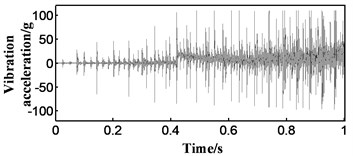
a) Zero drift signal

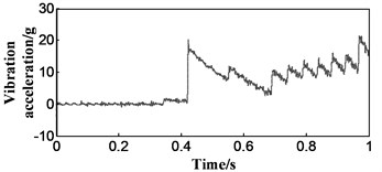
b) Drift trend term obtained by wavelet multi-scale decomposition: low frequency signal at seventh layer

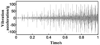
c) Signal after the zero drift is eliminated

2.2. Selection of the length of the time window

The selection of the length of the time window is very important in the analysis of vibration signals. The speed range of the diesel engine is generally between 600 rpm and 3000 rpm. Taking the four-stroke diesel engine as an example, with a sampling frequency of $f_{s}$ , the time for each revolution is given by $60 / v$ , where $v$ is the engine speed. The firing time interval derived from the ignition sequence of the engine, $t$ , and the number of sampling points within the time $t$ , $N_{0}$ ,are given by Eqs. (1) and (2), respectively:

1

t = \frac{120}{v n},

2

N_{0} (n, v) = f_{s} \times t = \frac{120 f_{s}}{v n},

where $n$ is the number of cylinders of the diesel engine.

Since the vibration signal is subjected to autocorrelation analysis thrice, it is necessary to ensure that the length of the vibration signal in each time window is sufficiently short and that the data length of the time window is sufficient for autocorrelation analysis, as shown in Eq. (3):

3

N_{0} \in (N_{0} (n, 3000), N_{0} (n, 600)) .

To ensure the accuracy of speed calculation, at least three main peaks must be retained after the three autocorrelation analyses. Therefore, the number of sample points in each time window must be as shown in Eq. (4):

4

N \geq 5 \times N_{0} (n, 600) .

2.3. Hilbert envelope of vibration signal

The most periodic representation of a vibration signal is the signal near its peak. In order to strengthen this part of the signal, we use Hilbert envelope for vibration signal processing.

Hilbert transform is an important means of signal processing. The Hilbert transform is used to transform the real signal into an analytic signal whose modulus is the Hilbert envelope signal. Hilbert transform can extract the instantaneous parameters of short signal and complex signal more effectively, which is helpful to analyze the vibration signal of diesel engine under unsteady conditions. The method that extracts the real signal envelope by Hilbert transforms is shown as follow:

5

ς (t) = s (t) + j \hat{s} (t),

6

\hat{s} (t) = H \{s\} = h (t) * s (t) = \int_{- \infty}^{\infty} s (τ) h (t - τ) d t = \frac{1}{π} \int_{- \infty}^{\infty} \frac{s (t)}{t - τ} d τ,

7

E (t) = |ς (t)|,

where $s (t)$ is the real signal, $\hat{s} (t)$ is the Hilbert transform of $s (t)$ , $ς (t)$ is the analytic signal, and $E (t)$ is envelope signal obtained.

In order to improve the signal to noise ratio (SNR), the engine vibration signal is analyzed using the Hilbert transform (Fig. 2). The envelope analysis highlights the main spike characteristics of the original signal well, greatly increasing the proportion of “interest” data in the signal.

Fig. 2Contrast between signals before and after envelope analysis

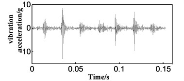
a) Signal before the envelope

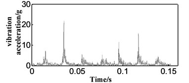
b) Enveloped signal

2.4. Calculation of the period of vibration by cubic autocorrelation

The engine speed in the vibration signal is reflected in the vibration signal cycle. The autocorrelation analysis is a powerful tool for analyzing the signal periodicity. Therefore, the analysis of the envelope signal by autocorrelation method can be used to analyze the period in the engine vibration signal.

The autocorrelation analysis is to calculate the similarity of the same data by means of the coordinate movement. The autocorrelation function is the correlation between the signal $x (t)$ and its own, as shown in Eq. (8):

8

R x x (t, τ) = E [x (t) x (t + τ)] = \underset{T \to \infty}{l i m} \frac{1}{T} \int_{0}^{T} x (t) x (t + τ) d t .

Vibration signals can be briefly represented as follows: $x (t) = s (t) + n (t)$ , where $s (t)$ is a useful signal, and $n (t)$ is a noise signal.

The autocorrelation function of the vibration signal is shown in Eq. (9):

9

R x x (t, τ) = E [x (t) x (t + τ)] = E [(s (t) + n (t)) (s (t + τ) + n (t + τ))]

= R s s (t, τ) + R s n (t, τ) + R n s (t, τ) + R n n (t, τ) .

Since the noise signal is not related to other signals, therefore $R s n (t, τ) = 0$ , $R_{n s} (t, τ) = 0$ :

10

R_{x x} (t, τ) = R_{s s} (t, τ) + R_{n n} (t, τ),

11

{R_{x x}}^{(2)} (t, τ) = E ((R_{s s} (t, τ_{1}) + R_{n n} (t, τ_{1})) (R_{s s} (t, τ_{1} + τ) + R_{n n} (t, τ_{1} + τ)))

= R_{s s} (R_{s s} (t, τ_{1})) + R_{n n} (R_{n n} (t, τ_{1})) = {R_{s s}}^{(2)} (t, τ) + {R_{n n}}^{(2)} (t, τ) .

Then the $i$ -times autocorrelation of the signal can be expressed as Eq. (12):

12

{R_{x x}}^{(i)} (t, τ) = {R_{s s}}^{(i)} (t, τ) + {R_{n n}}^{(i)} (t, τ) .

Since $n (t)$ is a random noise, the higher the number of correlation functions, the more obvious the noise reduction effect.

In order to find the most suitable autocorrelation number, a simulation signal with frequency of 10 Hz is constructed, in which the Gauss noise is added to analyze the frequency spectrum. The experimental results show that the more the number of autocorrelation, the better the noise reduction effect. When three autocorrelation operations are carried out, the noise has been greatly weakened (see Fig. 3).

Then we analyze the actual signal of the engine (see Fig. 4). As we can see in Fig. 4, where the engine vibration signal is analyzed by three autocorrelation analyses, the periodicity of the correlation curves is obvious. When the offsets of the first three peaks are defined as $l_{1}$ , $l_{2}$ , and $l_{3}$ , the vibration period and engine speed are as follows:

13

τ (k) = l_{3} / 3,

14

v (k) = 20 f_{s} / τ (k),

where $k$ is the number of the currently solved speed point.

Fig. 3Spectral contrast of autocorrelation with different times

a) Spectrum of simulated signal without noise

b) Primary autocorrelation spectrum after adding noise

c) Twice autocorrelation spectrum after adding noise

d) Three times autocorrelation spectrum after adding noise

e) Four times autocorrelation spectrum after adding noise

Fig. 4Different degrees of autocorrelation function

a) Primary autocorrelation

b) Twice autocorrelation

c) Three times autocorrelation

d) Four times autocorrelation

2.5. Moving window method and generation of speed-time scatter diagram

After the analysis of a time window, the time window needs to be moved, to measure the speed value at different points in time. The value of the shift window is given by Eq. (15):

15

u (k) = \{\begin{array}{l} 0, & k = 1, \\ τ (k - 1), & k \neq 1 . \end{array}

The speed-time curve is composed of several critical speed points. Based on the assumption that the speed is stable in the short time window, the midpoint of the time window is used as the speed point. The values are as shown in Eq. (16):

16

\{\begin{array}{l} t_{k} = \frac{1 + N + \sum_{i = 2}^{k} u (i)}{f_{s}}, \\ v_{k} = \frac{20 f_{s}}{τ (k)} . \end{array}

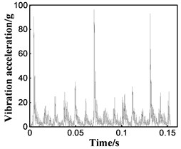
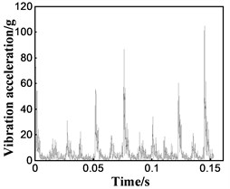
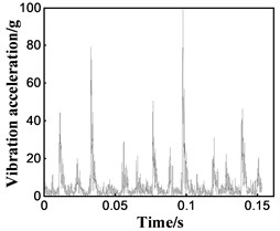
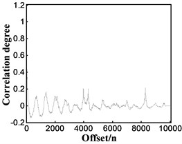
Fig. 5Processing details of speed measurement method under different engine working conditions

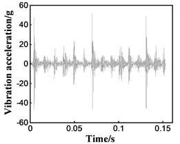
a1) Vibration signal after drifting zero drift (Normal)

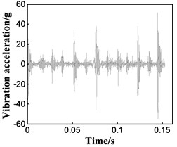
b1) Vibration signal after drifting zero drift (1 cutoff)

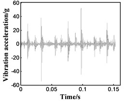
c1) Vibration signal after drifting zero drift (2-cutoff)

a2) Enveloped vibration signal (Normal)

b2) Enveloped vibration signal (1-cutoff)

c2) Enveloped vibration signal (2-cutoff)

a3) Primary autocorrelation (Normal)

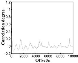
b3) Primary autocorrelation (1-cutoff)

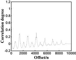
c3) Primary autocorrelation (2-cutoff)

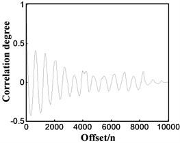
a4) Twice autocorrelation (Normal)

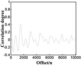
b4) Twice autocorrelation (1-cutoff)

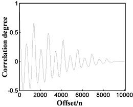
c4) Twice autocorrelation (2-cutoff)

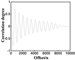
a5) Three times autocorrelation (Normal)

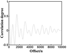
b5) Three times autocorrelation (1-cutoff)

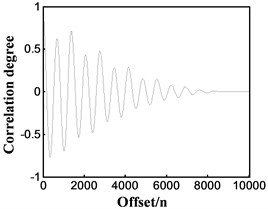
c5) Three times autocorrelation (2-cutoff)

The speed measurement method proposed in this paper is used to deal with the engine vibration signal under different working conditions, and the processing details are shown in Fig. 5, wherein “Normal” represents the engine in the normal state, “1-cutoff” represents the status of one cylinder being disable by cutting its oil off, and “2-cutoff” represents that of two cylinders.

2.6. Bench verification of speed measurement method

We verified the above-mentioned speed measurement method under no-load conditions. The full-condition test was carried out using the Weichai WD615 engine, and the acceleration sensor was installed. Rotational speeds were restored from vibration signal, which were validated by mounted rotational speed sensor. First, validation tests were carried out under normal steady-state conditions. We kept the engine speed fixed at values of 800 rpm, 1200 rpm, 1400 rpm, and 1600 rpm; the results are shown in Table 1.

Table 1Error values of rotational speed measurement under steady state

Real speed / (r·min^-1)	Calculated speed / (r·min^-1)	Error rate / (%)
800	804	0.5
1200	1205	0.42
1400	1407	0.5
1600	1604	0.25

Fig. 6Speed recovery under different non-stationary conditions

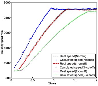
Fig. 7Speed recovery and error analysis under accelerated modes

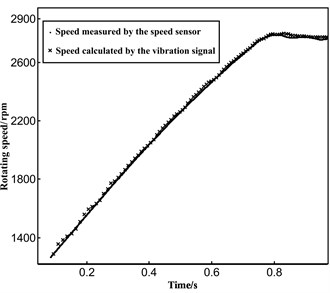
a) Speed recovery under rapid acceleration condition

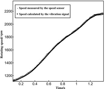
b) Speed recovery under slow acceleration condition

Then, the verification test was carried out under the condition of unsteady state. The non-stationary state used in the test is the acceleration state, which is reached by manually adjusting the accelerator pedal. When the throttle is fully open, the diesel engine speed under different conditions can be calculated as shown in Fig. 6. We also carried out the speed test under slow acceleration condition, as is shown in Fig. 7.

It can be seen from Fig. 6 and Fig. 7 that the values of rotational speed calculated by the algorithm are in good agreement with the real speed values, which meets the requirements of the engine rotational speed measurement accuracy under unsteady conditions. By analyzing the results of multiple tests, the maximum error of the algorithm under unsteady conditions is found to be 1.4 %, which accords with the accuracy requirements of rotational speed measurement.

3. Power measurement without external load

3.1. Principle of engine power measurement without external load

According to the basic principle of power measurement, power measurement without external load can be divided into two categories-one is the instantaneous power measurement, which is measured using the instantaneous angular acceleration, and the other is the average power measurement, which is measured using acceleration time. Instantaneous power detection requires the detection system to have the ability to process and calculate the speed signal of the speed sensor. In this paper, the acceleration time method is used to measure the average power.

Assuming the time when the engine crankshaft rotation angular velocity rises from $ω_{1}$ to $ω_{2}$ to be $Δ T$ , the average power of the engine, $\bar{P}$ , during this time is obtained as follows:

17

\bar{P} = \frac{A}{Δ T} = \frac{1}{2} J \frac{{ω_{2}}^{2} - {ω_{1}}^{2}}{Δ T},

where $J$ is the moment of inertia in the engine. Obviously, $ω = n π / 30$ . If kilowatt (kW) is taken as the unit of average power, the average power can be computed as follows:

18

\bar{P} = \frac{C_{1}}{Δ T},

19

C_{1} = \frac{1}{2} J {(\frac{π}{30})}^{2} \frac{n_{2}^{2} - n_{1}^{2}}{1000} .

If the moment of inertia is known, and the starting speed $n_{1}$ and the terminal speed $n_{2}$ are determined, $C_{1}$ is a constant called the average power factor. In general, the starting speed should be slightly higher than the idle speed, and the terminal speed should be the rated speed.

The above formula shows that, if the moment of inertia $J$ is known, and $n_{1}$ , $n_{2}$ can be determined, the average power will be inversely proportional to the acceleration time.

3.2. Curve fitting and interpolation of discrete velocity points

The key to no-load power measurement is to obtain the acceleration time of the specified speed range accurately. Since the time resolution of the previously calculated velocity-time scatter is poor, the parameters required to calculate the power cannot be determined accurately from the speed-time scatter plot. In order to obtain the precise time corresponding to the specified speed from the discrete values during acceleration, we must fit the function of rotational speed. This can be achieved in two ways-curve fitting and interpolation. Curve fitting refers to trying to find a smooth curve that best fits the data. Curve fitting must describe the intrinsic relationship between the two variables, time and rotational speed, and should reflect the trends of these discrete data well [14]. Here, we must find a curve that fits the discrete points well, and then use the curve equation to obtain the final acceleration time. The curve fitting method mainly involves choosing a suitable curve type, carrying out the variable transformation, solving the linear equation, and finally transforming the linear equation into a function. In the field of system identification, the least squares method is the most commonly used method for curve fitting, because it is highly accurate and practical [14, 15].

Interpolation of the curve is a basic function. When the amount of data is not sufficient, data are added, and the added data must have credibility. A smooth curve is constructed using ordered value points so that the curve passes sequentially through the sampling points. There are many methods for curve interpolation, such as polynomial curve interpolation, cubic Hermit interpolation, cubic parametric spline interpolation, multinode spline interpolation, algebraic interpolation, circular spline interpolation, and quasi-interpolation [16-18]. The adaptive cubic B-spline curve interpolation based on error control can adjust the number of interpolation points according to a preset error [19]. Under the premise of ensuring the accuracy of interpolation, this method effectively compresses the data volume.

As can be seen from Fig. 6, the rotational speed curves of good-condition engines are approximately linear during acceleration. With increase in the number of fuel cutoff cylinders, the slope of the acceleration curve decreases gradually.

It can be seen from Fig. 6 that there is no exact functional relationship between the velocity and time discrete points. This paper presents the method of curve fitting and interpolation based on the least squares method, which is used to locate the starting and terminal rotation speed accurately. The preliminary comparison of fitting and interpolation is shown in Fig. 8.

Fig. 8Comparison between the acceleration section’s discrete points based on fitting and interpolation in the normal condition

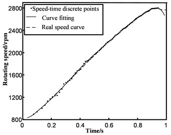
a) Cubic polynomial fitting

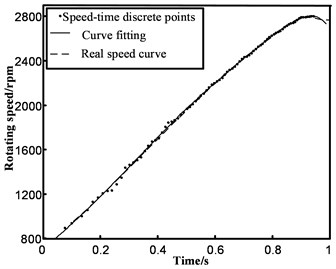
b) Third-order Gaussian fitting

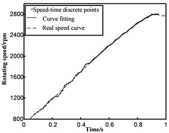
c) Cubic spline interpolation

d) Shape-preserving interpolation

The error analysis of several methods is shown in Fig. 9.

It can be seen from Fig. 9 that the reliability of the discrete point value is not sufficiently high, owing to the error factor of the velocity-time discrete point itself. This leads to a lower degree of approximation between the interpolation curve and the real speed curve, which is not as good as the effect of curve fitting, overall. Therefore, the curve fitting method based on least squares is used to fit the discrete points to obtain the acceleration time.

Fig. 9Error rate analysis of fitting curve and real velocity curve

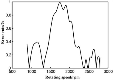
a) Cubic polynomial fitting

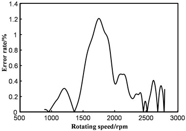
b) Third-order Gaussian fitting

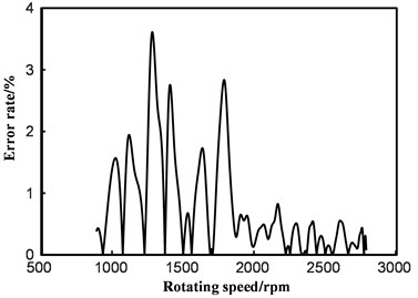
c) Cubic spline interpolation

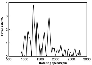
d) Shape-preserving interpolation

3.3. Optimal fitting scheme selection and power acquisition based on acceleration time

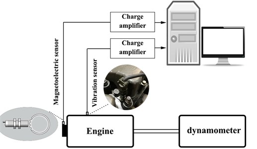
Acceleration time can be directly calculated from the equation of the fitted curve. It can be seen from Fig. 6 that the engine’s peak speed varies under different working conditions. In order to improve the stability of the actual work process, we selected the starting and terminal rotation speed values as 1000 rpm and 2600 rpm (rated speed) based on the previous experiences with no-load power measurement. The Weichai WD615 six-cylinder four-stroke diesel engine was tested on the bench, and the magnetoelectric sensor was mounted on the engine to achieve high-precision rotational speed in time, see Fig. 10. The speed discrete points from the vibration signal were analyzed in two different ways-fitting and interpolating. After comparing with the real acceleration time, we obtained the comparison of the fitting effects in different ways. It is shown in Fig. 11.

Fig. 10Experimental setup

It can be concluded from Fig. 11 that the average error rate of the curve fitting method is lower than that of the interpolation method; thus, the curve fitting method can be used to fit the discrete points. Among the different curve fitting methods, the 6th order polynomial, 7th order polynomial, and 4th order Gaussian fitting show good performances. In order to select the final fitting scheme, the accelerating tests of different groups are analyzed according to the practical needs of no-load power measurement, and the acceleration times of the three fitting methods are compared, as shown in Fig. 12.

Fig. 11Error rate comparison of different processing methods

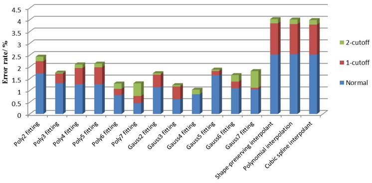
Fig. 12Contrasting the mean square errors of accelerated test errors of different fitting methods

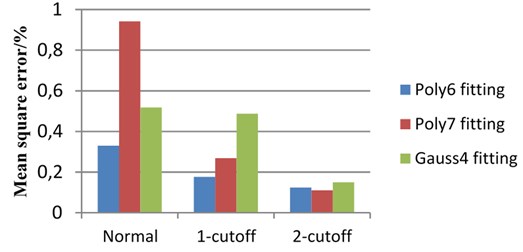
As can be seen in Fig. 12, the overall stability of the 6th order polynomial fitting is superior to that of the 7th order polynomial and the 4th order Gaussian fittings. Considering the comparisons of the different fitting methods in Fig. 11 and Fig. 12, the 6th order polynomial fitting is chosen as the final fitting method for velocity-time scatter. After repeated acceleration tests, the maximum error in the acceleration time in the method is controlled at 1.6 %.

By means of steady-state tests using a dynamometer, we obtained the moment of inertia of the engine and then calculated the average power using Eq. (18). We had calculated the average power, but it will change with the selected starting and terminal speed changes. Therefore, we chose the maximum power to describe the dynamic performance of the car. The two power values mentioned are different. However, researches show that there is a stable proportional relationship between the average power and the maximum power. Then, the maximum power can be calculated using Eq. (20):

20

P_{m} = K \bar{P},

where $K$ is the calibration coefficient, $\bar{P}$ is the average power calculated, and $P_{m}$ is the maximum power at engine rated speed.

We measured the maximum power under different operating conditions using a dynamometer, and then calibrated the average power obtained under no-load conditions. As the calibration coefficient was a fixed value, we used the least square method to deal with the calibration coefficients obtained from several experiments, and obtain the final calibration coefficient. As shown in Table 2, the error rates of maximum power recovery after calibration are less than 1.6 %, which can meet the accuracy requirement of power measurement.

Table 2Error rates of maximum power recovery after calibration under different working conditions

Running state of engine	Average power calculated by vibration signal /(kW)	Maximum power value after calibration /(kW)	Maximum power measured by the dynamometer /(kW)	Error rate/ (%)
Normal	127.87	187.8139	185.6	1.192
	126.00	185.0773	185.3	0.120
	124.64	183.0697	184.9	0.989
1-cutoff	98.14	144.1511	144.7	0.379
	97.78	143.6301	144.1	0.326
	100.0760	146.9887	144.9	1.441
2-cutoff	68.2592	100.2571	100.6	0.340
	67.8232	99.61672	100.1	0.482
	68.1538	100.1023	100.5	0.395

4. Conclusions

The speed-time scatter diagram was obtained from the vibration signals, using wavelet transforms, the Hilbert envelope, and three autocorrelations.

After comparing different curve-fitting and interpolation methods, the 6th order polynomial was chosen to fit the discrete points of the acceleration section. The acceleration time was obtained using analytical expressions. Finally, we obtained the maximum power through calibration tests. The main advantages of our proposed method are summarized below:

1) The method can measure the power without disassembling the vehicle, and hardware installation is convenient. The vibration sensor can be mounted at the top of any cylinder of the engine, and is suitable for vehicle diagnosis.

2) The algorithm is simple in structure, highly efficient, and has high accuracy in power measurement. The accuracy is 98.4 %, when using wavelet decomposition, envelope analysis, and cubic autocorrelation analysis combined with the curve-fitting technique, which meets the accuracy requirements of no-load power measurement.

References

Alisaraei A. T., Asl A. R. The effect of added ethanol to diesel fuel on performance, vibration, combustion and knocking of a CI engine. Fuel, Vol. 185, 2016, p. 718-733.

Publisher
Hassan-Beygi S.R., Istan V., Ghobadian B., et al. An experimental investigation of Perkins A63544 diesel engine performance using D-Series fuel. Energy Conversion and Management, Vol. 76, 2013, p. 356-361.

Publisher
Hua C. R., Dong D. W., Yan B., et al. Online monitoring ICE powers based on the crankshaft angular vibration. Applied Mechanics and Materials, Vols. 48-49, 2011, p. 773-778.

Publisher
Liu Y. J., Cai F. T., Zhou W., et al. An Engine Dynamic Signal Testing System Based on Virtual Instrument Technology. Applied Mechanics and Materials, Vol. 16, 2009, p. 193-198.

Publisher
Giebeler C., Adelerhof D. J., Kuiper A. E. T., et al. Robust GMR sensors for angle detection and rotation speed sensing. Sensors and Actuators A: Physical, Vol. 91, 2001, p. 16-20.

Publisher
Charles P., Sinha J. K., Gu F., et al. Detecting the crankshaft torsional vibration of diesel engines for combustion related diagnosis. Journal of Sound and Vibration, Vol. 321, Issue 3, 2009, p. 1171-1185.

Publisher
Lin H., Ding K. A new method for measuring engine rotational speed based on the vibration and discrete spectrum correction technique. Measurement, Vol. 46, Issue 7, 2013, p. 2056-2064.

Publisher
Urbanek J., Barszcz T., Antoni J. A two-step procedure for estimation of instantaneous rotational speed with large fluctuations. Mechanical Systems and Signal Processing, Vol. 38, Issue 1, 2013, p. 96-102.

Publisher
Xu J., Zhang G., Li B. Engine revolution speed measurement method based on single-point virtual vibration power. Chinese Journal of Scientific Instrument, Vol. 3, 2014, p. 697-702.

Search CrossRef
Diao Z., Quan H., Lan L., et al. Analysis and compensation of MEMS gyroscope drift. 7th International Conference on Sensing Technology (ICST), Wellington, 2013, p. 592-596.

Publisher
Du J., Li J., Feng K., et al. Zero drift random error compensating methods for MEMS gyros based on polynomial fitting algorithm. Chinese Journal of Sensors and Actuators, Vol. 29, 2016, p. 729-732.

Search CrossRef
Wang Y., Lu J., Ma T. A new zero drift signal processing method for penetration acceleration. Chinese Journal of Sensors and Actuators, Vol. 28, 2015, p. 510-514.

Search CrossRef
Beylkin G., Coifman R., Rokhlin V. Fast wavelet transforms and numerical algorithms I. Communications on Pure and Applied Mathematics, Vol. 44, 1991, p. 141-183.

Publisher
Giarnetti S., Leccese F., Caciotta M. Non recursive nonlinear least squares for periodic signal fitting. Measurement, Vol. 103, 2017, p. 208-216.

Publisher
Wang H. K., Ma J. S., Fang L. Q., et al. Application of the least squares support vector machine based on quantum particle swarm optimization for data fitting of small samples. Applied Mechanics and Materials, Vol. 472, 2014, p. 485-489.

Publisher
Lai M. J., Meile C. Scattered data interpolation with nonnegative preservation using bivariate splines and its application. Computer Aided Geometric Design, Vol. 34, 2015, p. 37-49.

Publisher
Stoyanov M. K., Webster C. G. A dynamically adaptive sparse grids method for quasi-optimal interpolation of multidimensional functions. Computers and Mathematics with Applications, Vol. 71, Issue 11, 2016, p. 2449-2465.

Publisher
Li C. Y., Zhu C. G. A multilevel univariate cubic spline quasi-interpolation and application to numerical integration. Mathematical Methods in the Applied Sciences, Vol. 33, Issue 13, 2010, p. 1578-1586.

Publisher
Ye T., Li X., Zeng Q. Adaptive curve interpolation of cubic B-spline based on error control. Computer Engineering and Applications, Vol. 49, Issue 1, 2013, p. 199-201.

Search CrossRef

Cited by

2023 International Conference on Control, Automation and Diagnosis (ICCAD)

Eli Gildish | Michael Grebshtein | Yehudit Aperstein | Igor Makienko

(2023)

About this article

Received

23 June 2017

Accepted

19 October 2017

Published

15 November 2017

SUBJECTS

Mechanical vibrations and applications

DOI

https://doi.org/10.21595/jve.2017.18788

Keywords

no-load power measurement

engine rotation speed detection

wavelet transform

Hilbert transform

autocorrelation

curve fitting

Acknowledgements

This work was funded by the Tianjin Natural Science Foundation (No. 15JCTPJC64200). Their support is acknowledged gratefully. We would like to thank Editage (www.editage.com) for English language editing. The authors declare that there are no conflicts of interest regarding the publication of this paper

This is an open access article distributed under the Creative Commons Attribution License, which permits unrestricted use, distribution, and reproduction in any medium, provided the original work is properly cited.

Previous article in issue Previous Next article in issue Next

Research article

2022 09 24

Railway foreign body vibration signal detection based on wavelet analysis

Chengjie Wei, Zhonghua Mu, Mohammed Wasim Bhatt

Research article

2019 09 30

Bearing fault diagnosis based on feature extraction of empirical wavelet transform (EWT) and fuzzy logic system (FLS) under variable operating conditions

Fawzi Gougam, Chemseddine Rahmoune, Djamel Benazzouz, Boualem Merainani

Research article

2018 09 24

Vibration signal de-noising based on empirical wavelet transform autocorrelation analysis

Jiajia Han, Jide Jia, Xiangyu Jia, Gang Ren

Research article

2017 12 31

Fault diagnosis of rotor using EMD thresholding-based de-noising combined with probabilistic neural network

Dong Liu, Hongtao Zeng, Zhihuai Xiao, Lihong Peng, O. P. Malik

S. Zhang and R. Zeng, “Engine power measurement without external load based on vibration signal,” Journal of Vibroengineering, Vol. 19, No. 7, pp. 4898–4910, Nov. 2017, https://doi.org/10.21595/jve.2017.18788

Copy Extrica

Copied to clipboard!

TY  - JOUR
DO  - 10.21595/jve.2017.18788
UR  - https://doi.org/10.21595/jve.2017.18788
TI  - Engine power measurement without external load based on vibration signal
T2  - Journal of Vibroengineering
AU  - Zeng, Ruili
AU  - Zhang, Shuai
PY  - 2017
DA  - 2017/11/15
PB  - JVE International Ltd.
SP  - 4898-4910
IS  - 7
VL  - 19
SN  - 1392-8716
ER  - 

Copy Ris

Copied to clipboard!

@article{Zeng_2017,
	doi = {10.21595/jve.2017.18788},
	url = {https://doi.org/10.21595/jve.2017.18788},
	year = 2017,
	month = {nov},
	publisher = {{JVE} International Ltd.},
	volume = {19},
	number = {7},
	pages = {4898--4910},
	author = {Ruili Zeng and Shuai Zhang},
	title = {Engine power measurement without external load based on vibration signal},
	journal = {Journal of Vibroengineering}
}

Copy Bibtex

Copied to clipboard!

[1]R. Zeng and S. Zhang, “Engine power measurement without external load based on vibration signal,” Journal of Vibroengineering, vol. 19, no. 7, pp. 4898–4910, Nov. 2017, doi: 10.21595/jve.2017.18788.

Copy IEEE

Copied to clipboard!

Zeng, Ruili, and Shuai Zhang. “Engine Power Measurement without External Load Based on Vibration Signal.” Journal of Vibroengineering 19, no. 7 (November 15, 2017): 4898–4910. https://doi.org/10.21595/jve.2017.18788.

Copy Chicago

Copied to clipboard!

Engine power measurement without external load based on vibration signal

Abstract

1. Introduction

2. Speed measurement based on vibration signals

2.1. Preprocessing of vibration signals

2.2. Selection of the length of the time window

2.3. Hilbert envelope of vibration signal

2.4. Calculation of the period of vibration by cubic autocorrelation

2.5. Moving window method and generation of speed-time scatter diagram

2.6. Bench verification of speed measurement method

3. Power measurement without external load

3.1. Principle of engine power measurement without external load

3.2. Curve fitting and interpolation of discrete velocity points

3.3. Optimal fitting scheme selection and power acquisition based on acceleration time

4. Conclusions

References

Cited by

About this article

Related Articles