Faulty bearing features by variational mode decomposition

1. Introduction

Early detection of bearing defects is crucial for the prevention of damage. Various signal processing techniques involving time, frequency, and statistical methods are used to detect and follow the progress of incipient faults. The extraction of meaningful information from vibration data is always challenging, especially due to the non-stationary phenomena at play and the presence of noise, which can mask interesting information and, as a result, data must be analyzed using different approaches [1]. Empirical Mode Decomposition (EMD) is one of the most popular signal processing techniques applied in analyzing the non-stationary phenomena and diagnosing faults in rotating machinery [2]. The basic idea here is to decompose any complex data set into multiple Intrinsic Mode Functions (IMFs). The major drawback of EMD is the mode mixing involved. To overcome this drawback, EEMD is proposed [3]. The key advantage of this method involves adding white noise with a suitable amplitude in order to get the expected signals. However, the definition of the value of the added noise amplitude in EEMD remains empiric, and at approximatively 20 %. Recently, a new method called “Variational Mode Decomposition” (VDM) was developed by Dragomiretskiy and Zosso [4], with the main goal of decomposing a multi-component input signal into a discrete set of quasi-orthogonal Band-Limited Intrinsic Mode Functions (BLIMFs). VMD is used in this paper to extract faulty bearing features, and its performances are compared with those of the EMD method.

2. The variational mode decomposition method

Variational Mode Decomposition VMD is used to decompose an input signal $x\left(t\right)$ into a number of band-limited intrinsic mode functions (BLIMFs) [4]. Each mode $u_k$ is mostly compact around a center pulsation ${\omega }_k$ (which must be determined) with the specific sparsity properties of its bandwidth in the spectral domain. For each mode, we compute the analytical signal in order to obtain a frequency spectrum. Then, the frequency spectrum is shifted to a baseband by mixing it with an exponential tuned to ${\omega }_k$. The bandwidth of each mode is assessed by means of an $H^1$ Gaussian smoothness of the shifted signal. The VMD is written as a constrained variational problem:

Subject to:

These equations may be addressed by introducing a quadratic penalty and Lagrangian multipliers. The augmented Lagrangian is given as follows:

where $\alpha$ is the balancing parameter of the data-fidelity constraint.

Eq. (3) can be solved with the Alternate Direction Method of Multipliers (ADMM) [6]. All the modes gained from solutions in the spectral domain are written as:

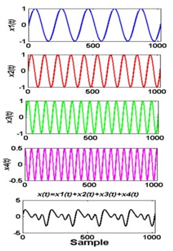
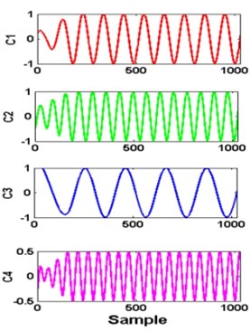
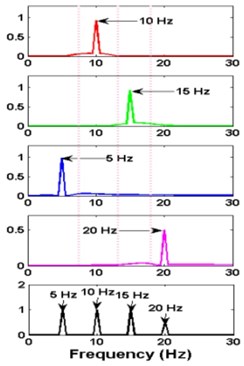
The original VMD algorithms may be found in [4]. Fig. 1 shows the result of a numerical signal containing 4 significant frequencies and alpha selected to 1000.

Fig. 1a) simulated signal xt and its components, b) signal decomposed by VMD, c) FFT of each mode: K= 4 and alpha = 1000

a)

b)

c)

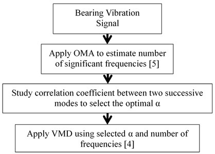
3. The proposed signal decomposition method: OMA-correlation-VMD

The proposed method is a hybrid method combining the OMA and VMD methods. The following steps are shown in Fig. 2.

Fig. 2OMA-Correlation-VDM method for extracting bearing frequencies

4. Experimental application to bearing defect diagnosis

4.1. Experimental setup

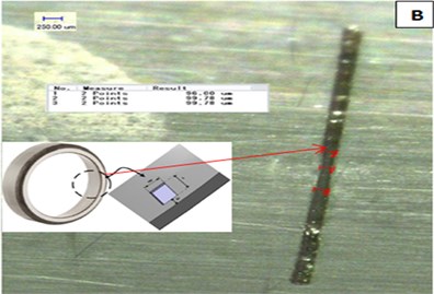
The experimental setup used in this study is shown in Fig. 3(a). It consists of a shaft mounted on two bearings and connected to a motor with a rubber coupling. The tested bearing was damaged by cutting a groove on the outer race using an electric discharge machine to control the size and depth (Fig. 3(b)). The depth of each defect was of the order of 200 µm. Different sizes ranging from 50 µm (early stage of degradation) to 2 mm (50 µm, 100 µm, 200 µm and 2 mm) were tested in order to extract the bearing defect frequencies at three degradation stages considered in this study. The first class corresponded to the healthy condition. The second class included a defective bearing at an early stage ranging from 50 μm to 200 μm, and the third class was an advanced defect of the order of 2 mm.

Fig. 3a) bearing test bench, b) defect on outer race

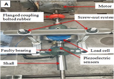
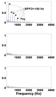
The signals were recorded with a PCB 352C34 accelerometer at a rotation speed of 1500 rpm (25 Hz) and a load of 6000 Newton. The load effect was applied by a screw-nut system. The sampling frequency was 48,000 Hz, and each recording was made with a precision of 0.2 Hz. The bearings used were ball bearing 1210 EKTN9 model. The symptomatic order of the bearing fault was BPFO at 7.24 (181 Hz).

4.2. Results and analysis

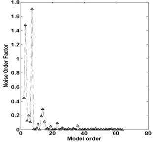
First, the ARMA method was applied to the recorded signals to estimate the number of modes required to apply the VMD. Fig. 4 shows a frequency stability diagram of the healthy bearing.

Fig. 4a) Noise order factor: healthy bearing, b) frequency stability diagram

a)

b)

This figure reveals the presence of three frequencies that stay stable with the order.

a) The correlation coefficient $r$ is the calculated for two successive modes at different alpha values (Fig. 5). The values of alpha were selected respectively to: 2000, 2000, 2000, 3000, and 1700.

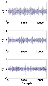
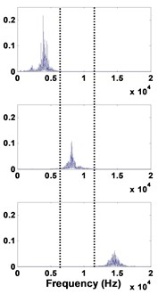
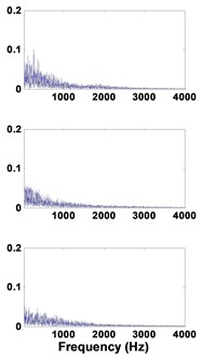
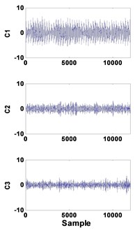
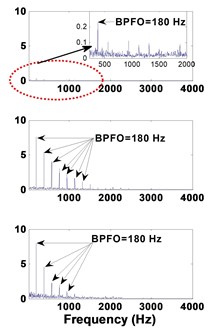
b) Finally, the VMD method was applied for extracting the main frequencies of the signal bearing using the number of modes estimated by OMA and alpha by the correlation coefficients. The results of the VMD decomposition are shown in Figs. 6-8 respectively for healthy bearing, 50 μm defective bearing, and 2 mm defective bearing.

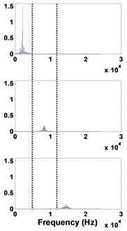
In the case of the healthy bearing, all modes, C1, C2 and C3 are, exempted from the BPFO frequencies. Fig. 6(b) shows that there is no mixing mode between all identified frequencies.

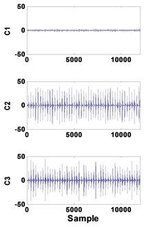
For the bearing at an early stage, the modes corresponding to the defective bearing is well extracted (C1), and the spectrum clearly shows the presence of BPFO peaks and its harmonics.

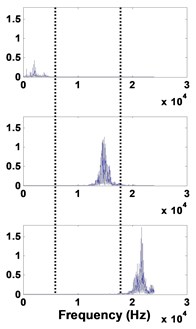
As expected for an advanced degradation, the fault excites all the bearing modes at high frequencies.

Fig. 5Correlation coefficients between two successive modes obtained by OMA: a) healthy bearing, b) for 50 µm, c) for 100 µm, d) for 200 µm and e) for 2 mm

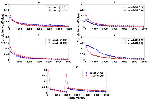
Fig. 6Healthy bearing: a) decomposed signal in time by VMD, b) frequency domain representation, c) spectrum of each mode

a)

b)

c)

Fig. 750 µm defective bearing: a) decomposed signal in time by VMD, b) frequency domain representation, c) spectrum of each mode

a)

b)

c)

Fig. 82 mm defective bearing: a) decomposed signal in time by VMD, b) frequency domain representation, c) spectrum of each mode

a)

b)

c)

5. Conclusions

This paper presents an adaptation of the “Variational Mode Decomposition” (VMD) method to be adaptively applied for the detection of faulty bearing frequencies. The required parameters (number of modes and balancing parameter alpha) have been solved by using the OMA method and a calculation of the correlation coefficients between two successive identified frequencies. The proposed method has been experimentally applied on measured vibratory signals on defective bearings. The results show that the OMA-correlation-VMD hybrid method can effectively detect the default frequencies and their harmonics.

References

-
Randall R. B., Antoni J. Rolling element bearing diagnostics – a tutorial. Mechanical Systems and Signal Processing, Vol. 25, Issue 2, 2011, p. 485-520.
Huang N. E., Shen Z., Long S. R., Wu M. L. C., Liu H. H. The empirical mode decomposition and the Hilbert spectrum for nonlinear and non-stationary time series analysis. The Royal Society, Vol. 454, 1998, p. 903-995.
Kedadouche M., Thomas M., Tahan A. Monitoring bearing defects by using a method combining EMD, MED and TKEO. Advances in Acoustics and Vibration, 2014, p. 502080.
Dragomiretskiy K., Zosso D. Variational mode decomposition. IEEE Transactions on Signal Processing, Vol. 62, Issue 3, 2014, p. 531-541.
Vu V. H., Thomas M., Lakis A. A., Marcouiller L. Operational modal analysis by updating autoregressive model. Mechanical Systems and Signal Processing, Vol. 25, 2011, p. 1028-1044.
Hestenes M. Multiplier and gradient methods. Journal of Optimization Theory and Applications Vol. 4, Issue 5, 1969, p. 303-320.
About this article
Financial support from the Natural Sciences and Engineering Research Council of Canada (NSERC) is gratefully acknowledged.