Hybrid spectral speed determination method for rotary machines

Gárdonyi, Gábor; Samu, Krisztián

doi:10.21595/jve.2018.19619

Journal of Vibroengineering

Browse Journal

Submit article

Published: 15 May 2019

Check for updates

Hybrid spectral speed determination method for rotary machines

Gábor Gárdonyi¹

Krisztián Samu²

^{1, 2}Department of Mechatronics, Optics and Mechanical Engineering Informatics, Budapest University of Technology and Economics, Budapest, 1111, Hungary

Corresponding Author:

Gábor Gárdonyi

Cite the article Download PDF

Abstract

Accurate rotational speed determination for rotary machines tends to be allocated high priority in technical applications. In some cases, it is not easy to measure shaft speed directly. Vibration diagnostic tools can offer an alternative solution to the problem posed by direct rotational speed measurement. Using calculated spectra and cepstra can help to determine the rotational speed easily and accurately. This paper examines the comparison of the spectrum and cepstrum based methods in terms of their applicable ranges and rotational speed estimation accuracy. Most papers which present similar comparisons state that the speed of rotary machines can be determined better with cepstrum calculation. However, this argument does not entirely stand up to scrutiny. This paper explains how to calculate the possible speed estimation error which arises out of the resolution of the discrete output data produced by the methodologies. The novel hybrid speed estimation logic uses these equations to decide which method results in the most accurate output. Numerous vibration measurements were made to test the usability of this hybrid method. It was successfully tested on electromotive drive trains, as well as spark- and compression-ignition internal combustion engines with different cylinder numbers and arrangements.

1. Introduction

It is often a critically important task to define an accurate, and measurement based method for estimating the operational state of the examined device. Rotational speed should ideally be measured for a high number of diagnostic algorithms, control or regulation processes. Incorrect values could cause serious disturbances in the operation of machines.

There are plenty of common rotational speed measuring solutions to solve this problem. One can easily use electrical, optical, magnetic [1] or combined [2] techniques as well. Other specific solutions which have been published to date include image processing techniques [3] and electrostatic sensors [4]. Speed fluctuations make traditional time based diagnostic tools difficult to use and less efficient. Angular sampling leads to have the same number of samples per rotation. It is then easier to use cyclostationarity diagnostic tools because the signal has periodic statistics as in the theory. Order tracking methods provide an interesting compromise to direct angular sampling. [5] Order tracking is the process of re-sampling the acquired signal in the angular domain and can be performed using hardware or software methods with very good accuracy [6].

The question of how one could measure the key parameters of an operating machine, particularly the rotating speed if the engineers did not perform these measurements in the early stages of design may arise. Mounting sensors into a device is usually not an easy task, in particular if doing so requires the modification of a rotating component. The difficulty is mainly caused by the compactness of modern devices. These parts are usually not directly accessible to users and there tends to be insufficient free space near the drive. In these instances vibration diagnostics that uses additional acceleration sensor and spectral analysis methods can be the best alternative solution [5-7]. Installation of speed sensors is not only expensive but straightforward impossible in some cases, for example because of the robust design of a coal harvester or if data series have previously been acquired without speed sensor information. In these cases vibration signal itself can be used to extract the missing speed. Further literature and examples about vibration based speed estimation of gearboxes, wind turbines, mining equipment, conveyors, jet engines, bearings, etc. can be found in Refs. [5-9]. Ref. [7] introduces a rolling element bearing diagnosis method where the synthesized tachometer signal is based on the bearing fault frequency instead of the rotational frequency. Traditional signal processing and feature extraction methods such as root mean square, kurtosis, peak magnitude and characteristic frequency estimation based, as well as an empirical mode decomposition based method are all introduced and compared to each other in Ref. [7]. Vibration signal analysis is nowadays the most commonly used method for troubleshooting and condition monitoring of rotary machines [6, 8].

This paper presents the development of a spectrum and cepstrum based hybrid calculation method. A new evaluation criteria has been set up for automatically selecting spectra or cepstra to determine the rotational speed. This method is capable of calculating the rotational speed of rotary machines more accurately than any of the aforementioned methods when used alone.

In the last few decades, spectrum [5-7, 9-12] and cepstrum [10, 13-15] based methods used for rotational speed and malfunction analysis have attracted much attention from research teams. However, to the authors’ best knowledge, there are very few publications available that discuss and compare the reliability of these two calculation methods [10, 15]. In the case of data acquisition systems, most of the settings are usually constant during a single measurement process. The two most relevant parameters are the sampling frequency and the buffer size of the data acquisition. It is possible to create equations based on these parameters which show whether the spectra or the cepstra calculation method produces a lower level of speed estimation error. The analyzed error originates from the resolution of output data series produced by each the two methods. This article explains how to calculate the applicable ranges, as well as the main decision levels which will assist in determining to use the preferable methodology.

2. Speed determination using spectrum and cepstrum calculation

2.1. Spectrum calculation

Traditional spectral analysis is concerned with the study of how the power of a signal is distributed in the frequency domain. After decomposing the original data series into sinusoidal components, it is relatively easy to detect a power content that corresponds to the rotational frequency [5-8, 14]. The $x$ coordinate of this peak represents the main operational frequency. In order to appreciate all of the detected frequency peaks one has to gain a thorough understanding of how the analyzed assembly works. In the case of a simple rotary machine the rotating speed can be determined directly from spectral results. Conversely, for internal combustion engines the periodic activity of the cylinders provides the dominant frequency [11]. Before any frequency analysis is undertaken it is necessary to clarify which part of the assembly is the dominant source of vibration.

The so-called APS (Auto Power Spectrum) is perhaps the most commonly used method in spectrum calculations. To estimate the APS, the DFT (Discrete Fourier Transformation) of the signal is computed and then multiplied by its complex conjugate [10]. Hence the magnitude of an APS is equal to the square magnitude of a DFT.

The theory of Fourier Transformation (FT) was originally developed for continuous signals. It is certainly possible to expand this theory to discrete time signals. The discrete equations are as follows:

1

D F T \{x [n]\} \equiv X [k] = \frac{1}{N} \sum_{n = 0}^{N - 1} x [n] e^{- i \frac{2 π}{N} k n}, k = 0,1, 2, . . ., (N - 1),

2

X [k] = \sum_{n = 0}^{N - 1} x [n] c o s (\frac{2 π}{N} k n) - i \sum_{n = 0}^{N - 1} x [n] s i n (\frac{2 π}{N} k n),

3

P [k] = R e {(X [k])}^{2} + I m {(X [k])}^{2},

where $P$ [ $k$ ] is the discrete APS, $X$ [ $k$ ] is the DFT of the $x$ [ $n$ ] discrete source signal.

During spectral analysis, signals are usually cut first into smaller pieces where overlapping and windowing can be applied. After the spectral calculation has been completed for every separate data series, it becomes possible to draw more reliable conclusions based on the averaged result. Alternatively, spectral analysis can also be calculated without averaging. However, averaging is a very effective method for eliminating random noises in case of stochastic processes and getting a smoother output.

2.2. Cepstrum calculation

Cepstrum was originally defined as the power spectrum of the power spectrum’s logarithm. Later, a newer definition was coined; cepstrum being the inverse transform of the power spectrum’s logarithm [13-15], expressed mathematically as:

4

c [n] = I D F T (l o g {|D F T \{x [n]\}|}^{2}) .

Commentators distinguish between four basic kinds of cepstral representation. These are the real, complex, power and phase cepstra [10].

A detailed study of the calculation methodology used for discrete data series and the particulars of the cepstral results can be found at Ref. [16]. For a number of further studies on the history and the application of cepstrum analysis please see the following references [10, 13-15, 17-19].

This method converts the signal into so-called quefrency components. One of the earliest applications of cepstrum theory can be found in the study of signals containing echoes and in the study of speech analysis. The application discussed in these studies was aimed at detecting the harmonic structure of measured sound. Such harmonic structures, so-called harmonic families, can be detected by gearbox analysis or, alternatively by any kind of analysis of rotary machines. The cepstrum calculation of a signal will only result in an evaluable output if its spectrum contains harmonic families as it searches for periodic changes in the spectrum. The latter is due to the cepstra’s behavior being similar to autocorrelation. This is to be expected in the light of the previously introduced definition of cepstrum, and when comparing Eq. (4) with the following mathematical definition, where $R_{x x}$ [ $n$ ] is the autocorrelation of $x$ [ $n$ ] signal [13, 15]:

5

R_{x x} [n] = I D F T ({|D F T \{x [n]\}|}^{2}) .

Similarly, to autocorrelation cepstrum output reveals nothing about absolute frequency only about the spacing of spectral peaks. The cepstrum data series’ variable possesses the dimensions of time, but is mostly referred to as quefrency. Before interpreting quefrency any further, it must be clarified that while the low quefrencies show slow changes in the spectrum, the high quefrencies correspond to rapid spectral fluctuations [13]. Usually the most dominant peak after the noisy fraction, belongs to the rotational speed or the so-called main harmonic component. The quefrency value of this peak shows the main time period in seconds. The distance between two data points of the resulting data series equals to the sampling period of the source signal. By the time the lowest quefrencies are reached, the result is usually much noisier. This is the reason why the rotational speed estimation method becomes unreliable at very high speeds (i.e. at small rotating periods). As it has been explained previously by spectral analysis, overlapping and windowing should be applied. Doing so, coupled with the use of averaging methods, will make the result much smoother. The cepstral output can be improved by using zero padded windowed signals. This treatment minimalizes the aliasing effect of cepstra [16].

2.3. Main parameters used for further calculation

Most data evaluation systems are configured with fixed parameters. Undoubtedly, these fixed parameters can be changed in special applications during the measurement. However, most sampling devices do not support such change requests. It is useful to consider the following parameters as given properties of the sampling setup:

$N_{t}$ is the number of samples, equals to window length. It can also be the buffer size at hardware side which is flushed out and processed in one step. It is practical to pick this value as the power of two. $F_{S}$ specifies the sampling rate in samples per second. $d t$ is the sample period of the time-domain signal in seconds. $T$ is the duration of the time-domain signal in seconds which is used for the calculations in one step:

6

d t = \frac{1}{F_{S}},

7

T = \frac{N_{t}}{F_{S}} .

$f_{ω 1}$ is the rotational frequency of the measured device’s main shaft in Hertz. This is the wanted parameter that had been examined in every instance discussed throughout this paper. In some cases this frequency, or the corresponding quefrency peak, can be directly determined by evaluation. In particular, when dealing with internal combustion engines it is useful to search for the upper- or sub-harmonics of this frequency. These specific cases will be discussed later in this paper, with the calculation method amended accordingly.

$T_{ω 1}$ is the period time in seconds which corresponds to $f_{ω 1}$ :

8

T_{ω_{1}} = \frac{1}{f_{ω_{1}}} .

$n_{ω 1}$ is the rotational speed expressed in r/min (revolutions per minute). In many cases shaft speed is expressed in this form. In this paper the calculations have been restricted to show how to arrive at $f_{ω 1}$ . $f_{ω 1}$ is easily convertible to r/min using the following expression [11]:

9

n_{ω_{1}} = f_{ω_{1}} \cdot 60 .

2.4. Attributes of spectrum result

$d f$ is the sample period of the frequency-domain data series in Hertz:

10

d f = \frac{F_{S}}{N_{t}} = \frac{1}{T} .

$N_{f}$ is the number of data points in the result. In this paper authors defined this parameter for one-sided spectral output. If $N_{t}$ is an even number (the power of two is recommended) the two-sided spectra will contain the corresponding value at the Nyquist frequency. This is half of the source signal’s sampling frequency. If this value is dropped by creating a one-sided spectra the following equation can be established:

11

N_{f} = \frac{N_{t}}{2} .

$f_{S p e c t m i n}$ is the lowest frequency after the DC component that has a corresponding value in the spectral output. $f_{S p e c t m a x}$ is the highest frequency that has a corresponding value in the spectral output. It is now the last frequency point before Nyquist frequency:

12

f_{S p e c t m i n} = \frac{F_{S}}{N_{t}},

13

f_{S p e c t m a x} = d f \cdot (N_{f} - 1) = \frac{F_{S}}{2} - \frac{F_{S}}{N_{t}} = \frac{F_{S} \cdot (N_{t} - 2)}{2 \cdot N_{t}} .

2.5. Attributes of cepstrum result

$d q$ is the sample period of the quefrency-domain signal in seconds. $N_{q}$ is the number of elements in the cepstrum result:

14

d q = d t = \frac{1}{F_{S}},

15

N_{q} = \frac{N_{t}}{2} + 1 .

Next we introduce a new frequency parameter, which is called $f_{C e p s m i n}$ . This is the lowest frequency that has a corresponding value in the quefrency domain. This is the reciprocal of the location of the last quefrency data point (expressed in seconds). $f_{C e p s m a x}$ is the highest frequency that has a corresponding time period in the quefrency domain. This frequency, as well as much lower ones, cannot be analyzed effectively in practice. Due to several reasons the output is much noisier in the case of high frequencies:

16

f_{C e p s m i n} = \frac{1}{d q \cdot (N_{q} - 1)} = \frac{1}{T / 2} = 2 \frac{F_{S}}{N_{t}},

17

f_{C e p s m a x} = \frac{1}{d q} = F_{S} .

3. Hybrid speed determination method

The speed determination method is called hybrid method because it uses the calculated spectrum as well as the cepstrum if needed. The decision logic is based on calculating the possible error. This paper solely analyses the error which arises from the resolution of the discrete data series. Naturally, the described results can be improved by several methods. Improvements to the most well-known approaches, as well as new methods, are published every year [20]. Following the links below, a few more literature sources can be found on how to improve spectral results by interpolation methods [21-23], averaging [7, 9, 24] or phase difference based [25] methods. These fall outside the scope of this article. In the experiment described herein, the authors used solely a simple peak searching method for frequency estimation.

The consideration behind developing the novel hybrid speed determination method is yet to be made absolutely clear. Both the spectrum and cepstrum calculations result in an output with linear resolution. The problem begins with the different domain of the outputs. One of them has linear resolution in frequency domain, while the other one has linear resolution in quefrency domain. If we convert the $x$ -axis values to the same unit – for example, to r/min – the spectrum result remains in linear resolution because of the linear operation described in Eq. (9). On the other hand, in the case of cepstrum output, transformed values along the $x$ -axis have a continuously increasing distance from each other as we move in the direction of higher values. The exponential scale is caused by the reciprocal operation that is to be used when changing the quefrency values (sec) to frequency (Hz) or also to rotational speed (r/min). If we convert both data series to the function of frequency, a new notion, Relative Step Size (RSS) must be introduced. The RSS is a certain function of frequency. This value can be defined as the ratio of the location of a point along the frequency axis and its distance to the nearest point. This RSS value shows us by how much the searchable frequency will be decreased if a detected frequency peak slides one value downward along the $x$ -axis.

To the authors’ best knowledge, very few available publications discuss the issue of examining and resolving spectral and cepstral output data series. One of them discusses the autocorrelation of the spectrum instead of cepstrum [11] but they arrive at similar conclusions to one another. On the occasions where they arrive at a conclusion comparing the two methods, they write something similar to:

It should be noted that the frequency estimation (actually the reciprocal of the equivalent quefrency) is very accurate because it is the average of the sideband spacing over the whole spectrum’ [15].

However, the above is not true in every case. This becomes clear when we consider the above defined RSS value. The relative error level in the frequency determination will decrease with spectral analysis and will increase with cepstral analysis in the direction of the higher values on the frequency axis. We can also draw the curve of RSS values in the function of n. In later chapters the authors will discuss which parameters can modify these two curves. For the time being, Fig. 1 solely illustrates the importance of the RSS calculation and why the hybrid method was developed to optimize spectral based speed estimation methodology.

Fig. 1RSS in the function of speed for hybrid (black dashed), spectrum based (red) and cepstrum based (blue) methods

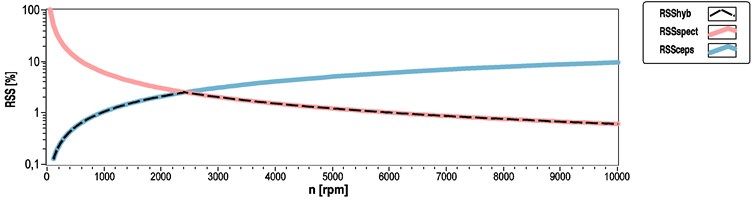
One of the questions is how to calculate the location of the intersection point of these two curves. This information will in turn provide the basis for the hybrid estimation method. At this point the next question we have to ask is the following: How can we decide on the calculation method for determining the queried frequency, if we have to make the decision based on the frequency itself?

Although cepstrum based analysis can provide us with the more accurate result, we will have to start the calculation with a spectrum calculation as can be seen from Eq. (4). As a side note, the experiment shows that when evaluating cepstrum results a simple search for the highest peak is insufficient for arriving at a reliable result. For an automated evaluation, we need to set search ranges because often the highest peak is not the queried one. However, the spectrum shows much more stability. If the analyzed physical process is well-known, it is usually not a major challenge to define the main frequency that will provide most of the power in the spectral result. If we can detect this main frequency peak and several harmonics, we can also detect the queried cepstrum peak in the close proximity of its corresponding quefrency. Therefore, we can determine an estimated frequency from the calculated spectrum which can hitherto be compared to the decision level of the hybrid method. If the estimated value is below the decision level, we can use the readily available two-sided spectrum data series for cepstrum calculation. If the estimated value is bigger than the decision level, we can save a lot of computational capacity without having to perform the cepstrum calculation. We can calculate the RSS value for the estimated frequency as well. If we have to use the cepstrum, it may be practicable to limit the quefrency range of the peak search proportional to the spectral RSS (e.g. multiplied by 1 to 3).

The following subsections show how to calculate the RSS in the function of frequency and the measurement’s main parameters. The paper also shows the calculation method for the spectrum and cepstrum based instances. Then the calculation of the intersection point will be deduced. The partial results are summarized later, in the Decision and applicable ranges of the hybrid method subsection, where the whole decision logic of the hybrid method can be found. In the equations the function of the RSS values is assigned as $E (f)$ .

3.1. RSS calculation of spectrum based method

The definition of RSS was introduced in the preliminary section of this chapter. Based on this definition Eq. (18) represents the way of calculating RSS for the spectral output:

18

E_{S p e c t} (f) = \frac{d f}{f} = \frac{F_{S}}{f \cdot N_{t}} .

The graphical representation of this function typically shows the shape of the falling curve in Fig. 1.

3.2. Referencing RSS calculation of the cepstrum based method

First, the function for the cepstrum based calculation must be defined. We can derive it analogously to the spectral instance of the quefrency domain, as shown in Eq. (19):

19

E_{C e p s} (T_{f}) = \frac{d q}{T_{f}} = \frac{1}{F_{S} \cdot T_{f}} .

In Eqs. (18) and (19) the RSS is defined as the function of different variables. To make these comparable we have to convert the argument of $E_{C e p s} (T_{f})$ to frequency. We shall define the above as Eq. (20):

20

E_{C e p s} (f) = \frac{1}{F_{S} / f} = \frac{f}{F_{S}} .

The typical shape of this function can be seen as the rising curve in Fig. 1.

3.3. RSS comparison of the methods

The above subsections show how to form equations for RSS calculation. Now, we can use Eq. (21) to determine the intersection point of the $E_{S p e c t} (f)$ and $E_{C e p s} (f)$ curves:

21

\frac{F_{S}}{f \cdot N_{t}} = \frac{f}{F_{S}},

22

\frac{{F_{S}}^{2}}{N_{t}} = f^{2},

23

f = \frac{F_{S}}{\sqrt{N_{t}}} .

Eq. (23) shows the location of the decision point along the frequency axis. It has been written as the function of the source signal’s sampling rate and the block size used for the evaluation. Usually these parameters are both constant throughout a measurement or evaluation process. This factor allows us to compute the decision frequency only once, at the beginning of the evaluation process. If the estimated frequency does not reach this level, we can make the final result more reliable using the cepstrum calculation:

24

f_{ω_{1}} < \frac{F_{S}}{\sqrt{N_{t}}} \to Cepstrum .

This decision frequency is applicable only if we are going to search the same frequency component using both methods. In addition, we must also appreciate the applicable ranges of each method.

3.4. Decision and applicable ranges of the hybrid method

The decision logic of the hybrid speed determination method is summarized in Eqs. (25) to (29), based on the previous calculations:

25

f_{ω_{1}} < \frac{F_{S}}{N_{t}} \to \begin{array}{l} Main frequency \\ not available, \end{array}

26

\frac{F_{S}}{N_{t}} \leq f_{ω_{1}} < 2 \cdot \frac{F_{S}}{N_{t}} \to Spectrum,

27

2 \cdot \frac{F_{S}}{N_{t}} \leq f_{ω_{1}} < \frac{F_{S}}{\sqrt{N_{t}}} \to Cepstrum,

28

\frac{F_{S}}{\sqrt{N_{t}}} \leq f_{ω_{1}} \leq \frac{F_{S} \cdot (N_{t} - 2)}{2 \cdot N_{t}} \to Spectrum,

29

f_{ω_{1}} > \frac{F_{S} \cdot (N_{t} - 2)}{2 \cdot N_{t}} \to \begin{array}{l} Main frequency \\ not available, \end{array}

The graphical representation of the corresponding RSS error curves and the resulting error of the hybrid method is illustrated by Fig. 1.

4. Using hybrid method for determining the speed of rotary machines

In the case of numerous rotary machines, searching upper or sub-harmonic component instead of the main frequency makes signal processing automation much easier and more reliable. For the purpose of these calculations we have to extend the aforementioned theory with two new parameters. These parameters depend on the structure of the analyzed device and the measurement’s layout (measured property, sensor position, orientation).

One of the new parameters has been named $p$ . The abbreviation originates in the ‘Number of Poles’ phrase. It shows the number of main parts in a structure that cause periodical vibration, acoustic noise or have any other measurable effect. Usually these are the driving parts of the machine that keep the shaft rotating. Most drives cannot grant an absolutely even torque and they cause pulsation in other parts too. If the torque has a really small deviation over time, we can usually find eccentric parts or cogwheels causing a certain, periodically changing effect. A few examples of how to determine the $p$ parameter for radial or tangential vibration measurement can be found below:

• Eccentric shaft: $p =$ 1;

• Electric motor: $p =$ Number of pole pairs;

• Internal combustion engine: $p =$ Number of cylinders.

The other new parameter has been named $r$ and originates in the ‘Number of Revolutions’ phrase. It shows how many revolutions are made by the main shaft during one whole period of the machine’s functionality. This parameter carries great importance, for example, for four-stroke internal combustion engines. Analogously to the $p$ parameter, below are some examples of how to determine this coefficient:

• Eccentric shaft: $r =$ 1;

• Electric motor: $r =$ 1;

• Four-stroke internal combustion engine: $r =$ 2.

The right definitions for the $p$ and $r$ parameters require prior analysis of the structural and measurement layout. If possible, we should also undertake some preliminary tests to verify their applicability.

The following deduction of the corresponding equations can be seen analogously to those in the former chapters; however, now extended with the $p$ and $r$ parameters.

4.1. RSS calculation of the spectrum based method for rotary machines

Direct detectable frequency component is $f_{ω S p e c t M a i n}$ . It can be expressed as:

30

f_{ω_{S p e c t M a i n}} = f_{ω_{1}} \cdot \frac{p}{r} = f_{ω_{p / r}} .

The definition of RSS was already introduced in Section 3. Eq. (18) showed the way of RSS calculation if the frequency of the detectable spectral component equals to the wanted frequency value. Now Eq. (31) shows the way of calculating RSS for the spectral output if the detectable and the searched frequencies differ from each other:

31

E_{S p e c t} (f_{ω_{1}}) = \frac{d f}{f_{ω_{p / r}}} = \frac{r \cdot F_{S}}{f_{ω_{1}} \cdot p \cdot N_{t}} .

4.2. RSS calculation of the cepstrum based method for rotary machines

In this case, directly detectable component in the cepstrum data series shows the $T_{ω C e p s M a i n}$ quefrency value which is proportional to the reciprocal of the corresponding $f_{ω C e p s M a i n}$ frequency component. Eqs. (32) and (33) show the definition of these components:

32

f_{ω_{C e p s M a i n}} = \frac{f_{ω_{1}}}{r} = f_{ω_{1 / r}},

33

T_{ω_{C e p s M a i n}} = \frac{r}{f_{ω_{1}}} = r \cdot T_{ω_{1}} = T_{ω_{1 / r}} .

As in Section 3.2, first, the simplest way of RSS calculation is defined by Eq. (34). Second, Eq. (35) shows the converted RSS function, where the argument becomes the wanted rotational frequency:

34

E_{C e p s} (T_{ω_{1}}) = \frac{d q}{T_{ω_{1 / r}}} = \frac{1}{r \cdot F_{S} \cdot T_{ω_{1}}},

35

E_{C e p s} (f_{ω_{1}}) = \frac{1}{r \cdot F_{S} \cdot \frac{1}{f_{ω_{1}}}} = \frac{f_{ω_{1}}}{r \cdot F_{S}} .

4.3. RSS comparison of the used methods for rotary machines

Based of the above subsections - by combining Eq. (31) and Eq. (35) – we are able to determine the value of $f_{ω 1}$ parameter at the point where the two error curves intersect each other:

36

f_{ω_{1}} = \frac{r \cdot F_{S}}{p \cdot \sqrt{N_{t}}} .

Eq. (36) shows the location of the decision point along the frequency axis. As in the case of Eq. (23), the formula contains only constant parameters. If the estimated rotational frequency does not reach this level, we can make the final result more reliable using the cepstrum calculation as shown by Eq. (37):

37

f_{ω_{1}} < \frac{r \cdot F_{S}}{p \cdot \sqrt{N_{t}}} \to Cepstrum .

As it has been already shown in Section 3, we must also appreciate the applicable ranges of each method.

4.4. Decision and applicable ranges of the hybrid method for rotary machines

The decision logic of the extended hybrid speed determination method is summarized in Eqs. (38) to (42), based on the above calculations. These extended formulas are applicable for any evaluation processes where the rotational frequency of the main shaft cannot be measured directly, but some other proportional frequency and quefrency components can be reliably detected:

38

f_{ω_{1}} < \frac{r \cdot F_{S}}{p \cdot N_{t}} \to \begin{array}{l} Main frequency, \\ not available \end{array}

39

\frac{r \cdot F_{S}}{p \cdot N_{t}} \leq f_{ω_{1}} < \frac{2 \cdot r \cdot F_{S}}{N_{t}} \to Spectrum,

40

\frac{2 \cdot r \cdot F_{S}}{N_{t}} \leq f_{ω_{1}} < \frac{r \cdot F_{S}}{p \cdot \sqrt{N_{t}}} \to Cepstrum,

41

\frac{r \cdot F_{S}}{p \cdot \sqrt{N_{t}}} \leq f_{ω_{1}} \leq \frac{r \cdot F_{S} \cdot (N_{t} - 2)}{2 \cdot p \cdot N_{t}} \to Spectrum,

42

f_{ω_{1}} > \frac{r \cdot F_{S} \cdot (N_{t} - 2)}{2 \cdot p \cdot N_{t}} \to \begin{array}{l} Main frequency \\ not available . \end{array}

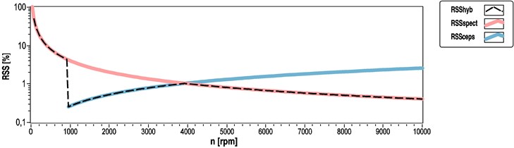
Fig. 2 represents an example of the modified RSS error curves, achieved through the extended equations if $p$ > $r$ > 1.

Fig. 2Parameterized RSS error in the function of speed for hybrid (black dashed), spectrum based (red) and cepstrum based (blue) methods

5. Joint time-frequency and time-quefrency analysis

As mentioned above, the output of spectrum and cepstrum can be smoothed using average calculation methods. Whilst linear weighting performed during a steady state analysis usually produces a better result, logarithmic weighting is much preferred for unsteady states or for real-time applications.

The spectra or cepstra calculated for the windowed signal sections can also be used for analyzing the coefficients’ changes over time. This consideration leads to the Short-Time Fourier Transformation (STFT). Eq. (43) demonstrates the discrete calculating method of the STFT [26]:

43

S T F T \{x [n]\} \equiv X (n, k) = \sum_{m = - \infty}^{\infty} x [m] w [n - m] e^{- j \frac{2 π}{N} k m},

where $x$ [ $n$ ] show the source signal, $w$ [ $n - m$ ] represent a real and even window, $S T F T$ { $x$ [ $n$ ]} is considered to be the output of the Short-Time Fourier Transform. We can display the result of this two-variable function as a three-dimensional output, usually called spectrogram. The interpretability of the results obtained through STFT will always be dependent on a compromise. With a large window size we get a high frequency resolution. The larger the window size, the more accurate the rotational speed which can be determined using the time-frequency representation. On the other hand, when using a small window size, the localizability over time will become better. It then becomes possible to observe or analyze transient processes due to the better resolution over time. More detailed information about STFT and the results of further improvement researches have been published under the following references [26-29]:

• By analogy with STFT, we can define an algorithm to examine the cepstrum changes over time. These graphs are usually called cepstrograms, where the resolution along the quefrency axis is not influenced by the window size. Instead, it solely depends on the sampling rate of the source signal.

• Both of the aforementioned STFT and TCA methods result in three dimensional outputs and also can be displayed using colormap, surface graphs or waterfall graphs as well. The result of hybrid analysis cannot be displayed in surface graphs if the hybrid method changes the type of background calculations during the evaluation process. At the change-point information content and the unit of coefficients will all change. If just the final result of the speed determination is used for display, we can easily change the background method if necessary. The displayed curve will not have any significant discontinuity at this point.

6. Using the hybrid calculation method in practice

The hybrid speed determination method was tested on several rotary machines to test its reliability. The hybrid method was tested through post-processing and real-time data evaluation application as well. The test applications were vibration acceleration measurements where a PCB356A33 3D accelerometer was fastened onto the surface of the analyzed devices by screw. Comparability of the acquired data series in different directions was increased with simultaneous sampling techniques for each channel, ensured by the application of the NI 9234 data acquisition card. The analyzed devices were connected to an adjustable load.

This paper intends to introduce the hybrid spectral method. Detailed description of real applications is neither an object nor feasible in this article.

6.1. Speed determination of a diesel engine

Figs. 3 and 4 show the measurement setup of the analyzed four-stroke four-cylinder compression ignition engine. We had to use $p =$ 4 and $r =$ 2 parameters for hybrid evaluation. The results of two measurements are shown in this paper.

The first three graphs (Figs. 5-7) show the data evaluation results achieved through the three speed determination methods for the vibration signal sampled at 51.2 kHz. The applied window size was 16384. To examine the simplest solution, no overlap between neighboring windows has been applied. These parameters cause an estimated rotational speed value in every 0.32 s based on Eq. (6) where the outputs $F_{S}$ parameter equals to 51.2 kHz divided by 16384. This section of the measurement contained a transition state from 1500 rpm speed to a lower speed of 1200 rpm.

Fig. 3Engine test bench with the straight-4 compression-ignition engine

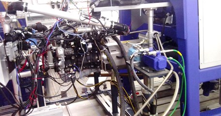
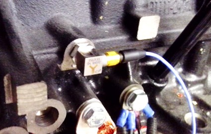
Fig. 4Mounted 3D accelerometer on the straight-4 compression ignition engine

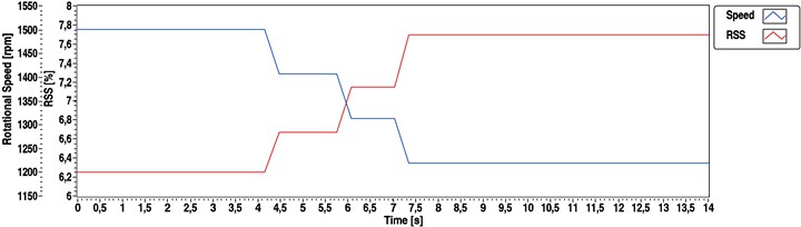
In Fig. 5 determined rotational speed values show only four levels of determined speed. At the beginning, the figure shows rotational speed of 1500 rpm until 4.1 s. The graph shows 1406.25 rpm determined speed between time instances 4.42 s and 5.70 s. 1312.5 rpm appears until 6.98 s. After 7.30 s only rotational speed values of 1218.75 rpm can be found. The size of drops in the determined speed values can be calculated based on Eq. (10). The absolute frequency step size becomes $d f =$ 3.125 Hz in this case which equals to $d n_{S p e c t} =$ 93.75 rpm according to Eq. (9). RSS values for the first seconds of this measurement can be calculated as $E_{S p e c t}$ ( $f_{ω 1} =$ 25 Hz) = 0.0625 = 6.25 % using Eq. (31).

Fig. 5Speed determination results calculated by the spectral method for a straight-4 compression-ignition engine (1500 to 1200 rpm transient)

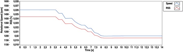
Cepstrum based algorithm gives much higher output resolution when using the same parameters (Figs. 6 and 7). RSS calculation for cepstrum based method can be carried out using Eq. (35). For the presented case $E_{C e p s}$ ( $f_{ω 1} =$ 25 Hz) = 0.000244 = 0.0244 %. This RSS level equals to $d n_{C e p s} =$ 0.366 rpm absolute step size based on Eq. (9).

Fig. 6Speed determination results calculated by cepstral method for a straight-4 compression-ignition engine (1500 to 1200 rpm transient)

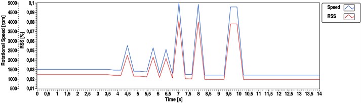
Fig. 7Speed determination results calculated by hybrid method for a straight-4 compression-ignition engine (1500 to 1200 rpm transient)

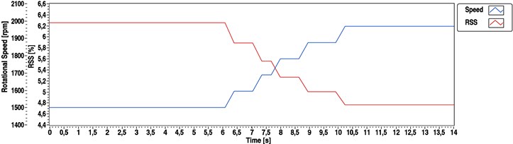
Figs. 8-10 show the evaluation results for another measurement of the same engine, where during the transition state the speed was raised from 1500 to 2000 rpm. In this case sampling frequency of the source signal was 6.4 kHz and a 2048 samples long window was used. This parameter set leads to the same time resolution of the output data because the ratio of the source signals sampling frequency and the applied window size remained the same. Time increment equals to 0.32 s without window overlapping, $d n_{S p e c t}$ is 93.75 rpm. However, cepstrum based methods (Figs. 9 and 10) show higher RSS value due to lower sampling frequency of the source signal. 1/8 of sampling frequency occurred 8 times greater RSS value in the output: $E_{C e p s}$ ( $f_{ω 1} =$ 25 Hz) = 1.56 % and $d n_{C e p s} =$ 2.928 rpm.

Fig. 8Speed determination results calculated by spectral method for a straight-4 compression-ignition engine (1500 to 2000 rpm transient)

In both transient cases, it could be observed that whilst the spectrum based estimation was really stable, it provided us through the applied parameters with a rather poor quality resolution. However, whilst the cepstral based method could offer a much better resolution, it appeared to be highly sensitive during the transient state. In this section of the measurement neither the quefrency peaks were sharp enough, nor was the loading torque steady enough. The automatic peak detection in the quefrency domain resulted in values with a rate of gross error. Contrary to these two simple methods, the hybrid estimation produced a nearly even and reliable output.

Fig. 9Speed determination results calculated by cepstral method for a straight-4 compression-ignition engine (1500 to 2000 rpm transient)

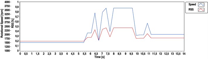
Fig. 10Speed determination results calculated by hybrid method for a straight-4 compression-ignition engine (1500 to 2000 rpm transient)

6.2. Speed determination of a DC drive

There is an advantage of the hybrid method; that it can switch the background algorithm during the evaluation process. This can be presented in the case of a measurement with larger speed transient processes. A representative example of such an evaluation is the DC drive analysis.

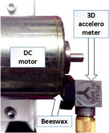
The test system consisted of a DC servomotor (Faulhaber 3557-K024-CS) connected to a hysteresis braking motor (HB-20M-2). A wheel with radial oriented black and white stripes was fixed to the end of the assembly’s driven shaft. Thanks to this striped wheel the angular movement could be detected with a single reflective optical sensor (Fig. 11). The piezoelectric accelerometer was mounted onto the housing surface of the DC servomotor with special beeswax (Fig. 12).

Fig. 11Optical rotational speed measurement of the driven braking motor

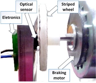
Fig. 12Vibration measurement of the analyzed DC motor which is connected to the braking motor

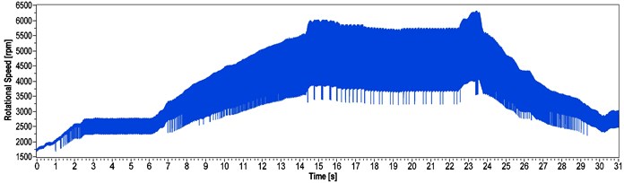
An advantage of the axle mounted striped wheel is that this way the rotational speed can be obtained with simplistic signal processing methods, and usually with good accuracy. Due to the mechanical structure – if the bearing is not suitable and the system leaves the proposed operational range – intensive vibration of the analyzed system could be observed. Because of this phenomenon a rate of gross error of encoder measurement occurred. As the striped wheel have left the operational range of the used optical sensor, there would have been undetectable stripes. Fig. 13 shows the fickleness of optical method above 2000 rpm rotational speed, due to the non-detected stripes of the wheel. In such instances the fault caused a level of up to 60 % relative error in the result. Though the encoder gave such noisy results, we could use the upper above envelope as a reference speed, by analyzing the vibration based method’s output.

Fig. 13Result of the encoder measurement of the DC drive between 1500 and 6500 rpm

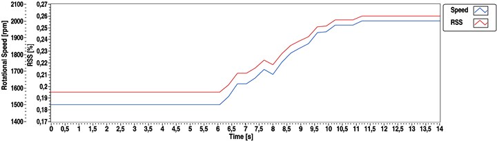
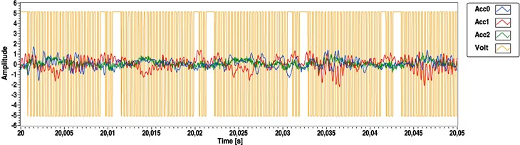
A section of the source signal from a steady state measurement in this high-speed range is interpreted in Fig. 14. The figure clearly shows that there were cyclically missing signal changes at a particular angular range.

Fig. 14Result of the encoder measurement of the DC drive between 1500 and 6500 rpm

The following figures show the outputs of the spectrum based (Fig. 15), cepstrum based (Fig. 16) and the hybrid (Fig. 17) speed determination methods. The measurement was the same as in case of Fig. 13. We could get the following results using the $p =$ 1 and $r =$ 1 parameters. During this measurement the eccentricity was the dominant source of vibration.

Fig. 15Speed determination of the DC motor using the spectral method

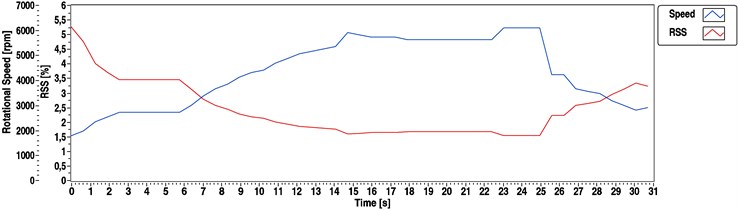
In this case 1.6 kHz sampling frequency and 1024 samples long window have been used. This parameter combination produces an output value in every 0.64 s. Based on Eq. (36) 3000 rpm decision level of the hybrid spectral methodology can be determined. At this point (near to 3000 rpm) both methods produce 3.125 % RSS which means an absolute step size of 1.56 Hz or 93.75 rpm.

Fig. 16Speed determination of the DC motor using the cepstral method

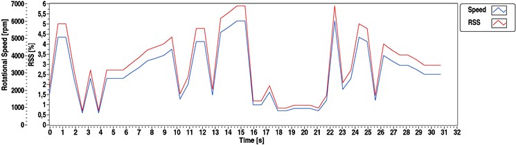
Fig. 17Speed determination of the DC motor using the hybrid method (background method changes at 3000 rpm)

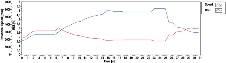
Almost the same observations could be made about the curves as in the previous instance: whereas the spectrum result was stable, the cepstrum result had a rate of gross error. However, if we have a look at the red RSS curve of the hybrid method, something different can be observed. As the hybrid method (Fig. 17) had to change its calculation mode at a 3000 rpm estimated rotating speed, the method always produced the final result with the lowest RSS level.

The experiments show that sensor orientation had great influence on the evaluation. The above formulas for the $p$ and $r$ parameters were not valid for axial vibration components. They were only applicable to vertical or cross-oriented accelerations. Using spectral speed estimation methods, we usually could not get specific information about speed fluctuation within one revolution of the rotary machine, but these methods are able to reproduce the average shaft speed within the calculated RSS level. The efficiency of spectrum based and hybrid methods was slightly influenced by the applied load contrary to the cepstrum based speed determination.

7. Conclusions

This article lays out a hybrid technique which improves common spectrum and cepstrum based rotating speed determination methods. This study discusses the way to calculate the representations’ RSS error parametrically. Based on that, a hybrid method has been developed which makes use of both methods. First, it calculates the applicable ranges of both methods and also a decision level to give the final result with the best resolution. Second, it calculates the spectrum of the sampled time series and searches the peak which corresponds to the rotational speed. Third, the algorithm compares the peak location to the calculated decision level. The decision point is proportional to the ratio of the sampling frequency to the square root of used FFT size. Fourth, the discrete cepstrum must be calculated at lower speed ranges. The theory and the equations have been also extended with new parameters for generalization and for a more efficient analysis of rotary machines. The hybrid method, with its extended background theory was tested on several rotary machines. The main conclusions around the method were as follows: (i) it can be used for numerous machine structures if the parameters are defined correctly; (ii) it provides the robustness of a simple spectral analysis, even when it uses the cepstral method for the determination of the final result (it will not be instable either at transient state analysis); (iii) it can switch between spectra and cepstra based methods during evaluation and always uses the method which provides the best resolution; (iv) even at relatively high rotational speeds it does not perform unnecessary calculations and the calculation duration is the same as for a common spectrum evaluation; (v) it can be used for post-processing and for real-time analysis as well.

References

Giebeler C., et al. Robust GMR sensors for angle detection and rotation speed sensing. Sensors and Actuators A-Physical, Vol. 91, 2001, p. 16-20.

Publisher
Didosyan Y. S., et al. Magneto-optical rotational speed sensor. Sensors and Actuators A-Physical, Vol. 106, 2003, p. 168-171.

Publisher
Zhang X., et al. Digital image correlation using ring template and quadrilateral element for large rotation measurement. Optics and Lasers in Engineering, Vol. 50, 2012, p. 922-928.

Publisher
Wang L. J., et al. Rotational speed measurement using electrostatic sensors with single or double electrodes. 2nd IET Renewable Power Generation Conference, 2013.

Publisher
Bonnardot F., et al. Use of the acceleration signal of a gearbox in order to perform angular resampling (with limited speed fluctuation). Mechanical Systems and Signal Processing, Vol. 19, 2005, p. 766-785.

Publisher
Urbanek J., et al. Comparison of amplitude-based and phase-based methods for speed tracking in application to wind turbines. Metrology and Measurement Systems, Vol. 18, 2011, p. 295-304.

Publisher
Siegel D., et al. Novel method for rolling element bearing health assessment – a tachometer-less synchronously averaged envelope feature extraction technique. Mechanical Systems and Signal Processing, Vol. 29, 2012, p. 362-376.

Publisher
Adams M. L. Rotating Machinery Vibration: From Analysis to Troubleshooting. Marcel Dekker, New York, 2001.

Publisher
Urbanek J., et al. Application of averaged instantaneous power spectrum for diagnostics of machinery operating under non-stationary operational conditions. Measurement, Vol. 45, 2012, p. 1782-1791.

Publisher
Liang B., Iwnicki S. D., Zhao Y. Application of power spectrum, cepstrum, higher order spectrum and neural network analyses for induction motor fault diagnosis. Mechanical Systems and Signal Processing, Vol. 39, 2013, p. 342-360.

Publisher
Lin H., Ding K. A new method for measuring engine rotational speed based on the vibration and discrete spectrum correction technique. Measurement, Vol. 46, 2013, p. 2056-2064.

Publisher
Rodopoulos K., Yiakopoulos C., Antoniadis I. A parametric approach for the estimation of the instantaneous speed of rotating machinery. Mechanical Systems and Signal Processing, Vol. 44, 2014, p. 31-46.

Publisher
Randall R. B. Cepstrum Analysis and Gearbox Fault Diagnosis. Brüel & Kjaer, Naerum, 1980.

Search CrossRef
Li H., Zhang Y., Zheng H. Gear fault detection and diagnosis under speed-up condition based on order cepstrum and radial basis function neural network. Journal of Mechanical Science and Technology, Vol. 23, 2009, p. 2780-2789.

Publisher
Randall R. B. A history of cepstrum analysis and its application to mechanical problems. Surveillance 7th International Conference, Chartres, France, 2013, p. 1-16.

Search CrossRef
Childers D. G., Skinner D. P., Kemerait R. C. The cepstrum: a guide to processing. Proceedings of the IEEE, Vol. 65, 1977, p. 1428-1443.

Publisher
Brown J. D., Oliver J. The cepstrum: A viable method for the removal of ground reflections. Journal of Sound and Vibration, Vol. 71, 1980, p. 299-313.

Publisher
Kim J. T., Lyon R. H. Cepstral analysis as a tool for robust processing, deverberation and detection of transients. Mechanical Systems and Signal Processing, Vol. 6, 1992, p. 1-15.

Publisher
El-Ghamry M., et al. Indirect measurement of cylinder pressure from diesel engines using acoustic emission. Mechanical Systems and Signal Processing, Vol. 19, Issue 4, 2005, p. 751-765.

Publisher
Slepicka D., et al. Comparison of nonparametric frequency estimators. IEEE Instrumentation and Measurement Technology Conference Proceedings, Austin, 2010, p. 73-77.

Search CrossRef
Offelli C., Petri D. Interpolation techniques for real-time multifrequency waveform analysis. IEEE Transactions on Instrumentation and Measurement, Vol. 39, 1990, p. 106-111.

Publisher
Quinn B. G. Estimating frequency by interpolation using Fourier coefficients. IEEE Transactions on Signal Processing, Vol. 42, 1994, p. 1264-1268.

Publisher
Belega D., Dallet D., Petri D. Accuracy of sine wave frequency estimation by multipoint interpolated DFT approach. IEEE Transactions on Instrumentation and Measurement, Vol. 59, 2010, p. 2808-2815.

Publisher
Nuttall A. H., Carter G. C. A generalized framework for power spectral estimation. IEEE Transactions on Acoustics, Speech, and Signal Processing, Vol. 28, 1980, p. 334-335.

Publisher
Zhu L. M., et al. Noise influence on estimation of signal parameter from the phase difference of discrete Fourier transforms. Mechanical Systems and Signal Processing, Vol. 16, 2002, p. 991-1004.

Publisher
Kwok H. K., Jones D. L. Improved instantaneous frequency estimation using an adaptive short-time Fourier transform. IEEE Transactions on Signal Processing, Vol. 48, 2000, p. 2964-2972.

Publisher
Boashash B. Time-Frequency Signal Analysis and Processing. Elsevier, Brisbane, 2015.

Search CrossRef
Meltzer G., Ivanov Y. Y. Fault Detection in gear drives with non-stationary rotational speed – part I. Mechanical Systems and Signal Processing, Vol. 17, 2003, p. 1033-1047.

Publisher
Urbanek J., Barszcz T., Antoni J. A two-step procedure for estimation of instantaneous rotational speed with large fluctuations. Mechanical Systems and Signal Processing, Vol. 38, 2013, p. 96-102.

Publisher

Cited by

Application of Vibration Signal Processing Methods to Detect and Diagnose Wheel Flats in Railway Vehicles

JaeSeok Shim | GeoYoung Kim | ByungJin Cho | JeongSeo Koo

(2021)

About this article

Received

09 January 2018

Accepted

15 November 2018

Published

15 May 2019

SUBJECTS

Mechanical vibrations and applications

DOI

https://doi.org/10.21595/jve.2018.19619

Keywords

cepstrum

diagnostic

hybrid method

rotary machine

rotational speed

spectrum

This is an open access article distributed under the Creative Commons Attribution License, which permits unrestricted use, distribution, and reproduction in any medium, provided the original work is properly cited.

Next article in issue Next

Research article

2023 11 27

Analysis and prediction of automotive running status based on vibration detection system

Bo Yang, Yanchao Wang, Mei Yang

Review article

2021 11 26

Fault diagnosis and health management of bearings in rotating equipment based on vibration analysis – a review

Adnan Althubaiti, Faris Elasha, Joao Amaral Teixeira

Research article

2019 09 30

Bearing fault diagnosis based on feature extraction of empirical wavelet transform (EWT) and fuzzy logic system (FLS) under variable operating conditions

Fawzi Gougam, Chemseddine Rahmoune, Djamel Benazzouz, Boualem Merainani

Research article

2018 02 15

Rolling bearing fault diagnosis based on improved complete ensemble empirical mode of decomposition with adaptive noise combined with minimum entropy deconvolution

Abdelkader Rabah, Kaddour Abdelhafid

G. Gárdonyi and K. Samu, “Hybrid spectral speed determination method for rotary machines,” Journal of Vibroengineering, Vol. 21, No. 3, pp. 538–555, May 2019, https://doi.org/10.21595/jve.2018.19619

Copy Extrica

Copied to clipboard!

TY  - JOUR
DO  - 10.21595/jve.2018.19619
UR  - https://doi.org/10.21595/jve.2018.19619
TI  - Hybrid spectral speed determination method for rotary machines
T2  - Journal of Vibroengineering
AU  - Gárdonyi, Gábor
AU  - Samu, Krisztián
PY  - 2019
DA  - 2019/05/15
PB  - JVE International Ltd.
SP  - 538-555
IS  - 3
VL  - 21
SN  - 1392-8716
SN  - 2538-8460
ER  - 

Copy Ris

Copied to clipboard!

@article{G_rdonyi_2019,
	doi = {10.21595/jve.2018.19619},
	url = {https://doi.org/10.21595/jve.2018.19619},
	year = 2019,
	month = {may},
	publisher = {{JVE} International Ltd.},
	volume = {21},
	number = {3},
	pages = {538--555},
	author = {G{\'{a}}bor G{\'{a}}rdonyi and Kriszti{\'{a}}n Samu},
	title = {Hybrid spectral speed determination method for rotary machines},
	journal = {Journal of Vibroengineering}
}

Copy Bibtex

Copied to clipboard!

[1]G. Gárdonyi and K. Samu, “Hybrid spectral speed determination method for rotary machines,” Journal of Vibroengineering, vol. 21, no. 3, pp. 538–555, May 2019, doi: 10.21595/jve.2018.19619.

Copy IEEE

Copied to clipboard!

Gárdonyi, Gábor, and Krisztián Samu. “Hybrid Spectral Speed Determination Method for Rotary Machines.” Journal of Vibroengineering 21, no. 3 (May 15, 2019): 538–55. https://doi.org/10.21595/jve.2018.19619.

Copy Chicago

Copied to clipboard!

Hybrid spectral speed determination method for rotary machines

Abstract

1. Introduction

2. Speed determination using spectrum and cepstrum calculation

2.1. Spectrum calculation

2.2. Cepstrum calculation

2.3. Main parameters used for further calculation

2.4. Attributes of spectrum result

2.5. Attributes of cepstrum result

3. Hybrid speed determination method

3.1. RSS calculation of spectrum based method

3.2. Referencing RSS calculation of the cepstrum based method

3.3. RSS comparison of the methods

3.4. Decision and applicable ranges of the hybrid method

4. Using hybrid method for determining the speed of rotary machines

4.1. RSS calculation of the spectrum based method for rotary machines

4.2. RSS calculation of the cepstrum based method for rotary machines

4.3. RSS comparison of the used methods for rotary machines

4.4. Decision and applicable ranges of the hybrid method for rotary machines

5. Joint time-frequency and time-quefrency analysis

6. Using the hybrid calculation method in practice

6.1. Speed determination of a diesel engine

6.2. Speed determination of a DC drive

7. Conclusions

References

Cited by

About this article

Related Articles