Abstract
The timing belt drive is composed of a closed ring-shaped adhesive tape with corresponding teeth on the inner peripheral surface and corresponding pulleys. During exercise, the toothed teeth mesh with the pulley to transmit motion and power. The vibration problem of belt drive has always been a hot research topic. In order to analyze the vibration problem caused by belt drive, this paper makes use of the multi-body dynamics software RecurDyn belt drive simulation model. Through the model displacement sensor and the system simulation results, the various movement characteristics of the belt are analyzed.
1. Introduction
There are two main forms of vibration for belt drives [1]. The first is the vibration of the transmission system along the direction of the centerline of the two pulleys, that is, the longitudinal vibration of the belt drive. The second is the vibration of the belt along the direction perpendicular to the movement direction of the belt, namely the lateral vibration of the belt drive. Both forms of vibration will have a serious impact on the transmission characteristics of the belt drive, especially when the excitation frequency is close to the natural frequency of the belt drive system, the belt drive system will generate resonance, which may cause greater harm. Moreover, when the amplitude of the lateral vibration exceeds the safe range [2], the wear between the belt and the pulley will be aggravated, thereby affecting the service life of the belt.
In order to study the vibration characteristics of the timing belt, we used RecurDyn software to simulate the driving process of the timing belt, and analyzed the vibration characteristics of the belt drive through the data obtained from the simulation.
2. The basic algorithm of RecurDyn
In the belt drive system of the automobile, the pulley is a rigid body, the timing belt is a flexible body, so the timing belt drive system is a rigid-flexible hybrid system.
RecurDyn is the latest generation of multi-body system simulation optimization software developed by Korea’s FunctionBay based on recursive algorithm. It uses relative coordinate system motion equation theory and complete recursive algorithm, it is well suited for solving multibody dynamic problems with large-scale and complex contacts.
2.1. Coordinate system
The general movement of a rigid body in space is a continuum coordinate system that uses a certain point in a rigid body as the origin to create a rigid body. Any point in a rigid body is mathematically described with respect to point . As shown in Fig. 1, the posture of a rigid body can be expressed as:
where , , and are unit vectors along the , , and axes, respectively. The -- is a rigid body coordinate system and -- is an inertial reference coordinate system.
The speed and virtual displacement of the point defined in the -- coordinate system are:
The corresponding amount in the -- coordinate system is defined as:
Fig. 1Coordinates and rigid body
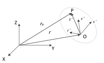
Fig. 2Kinematic relation of two adjacent members
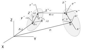
2.2. Relative movement of adjacent components
As shown in Fig. 2, there is a pair of adjacent components, let component () be the former component of the connection component (), and the position of the point is expressed as:
Defining , the angular velocity of component in its own reference coordinate system is given by Eq. (3):
where prime is determined by the axis of rotation.
Finding Eq. (4) subdivisions can be obtained:
The variable with a tilde symbol represents an oblique symmetric matrix consisting of vector elements in the vector cross product. Represents the relative coordinate vector. Substituting in Eq. (5) and multiplying both sides by a in Eq. (6) yields:
And . Simultaneously obtain the velocity recursive equations between the motions of adjacent components:
It is important to note that the matrices and are only the hinge relative coordinate functions of the connecting components () and ().
Similarly, the recursive relationship of virtual displacements is as follows:
3. The establishment of simulation model
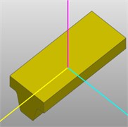
3.1. Create a 3D model
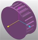
Open RecurDyn software and click to select the Belt Kit. First, select the TimingBelt, and set the parameters as shown in the Fig. 3.
Click to select the Pulley Timing, which is also set as shown in the figure.
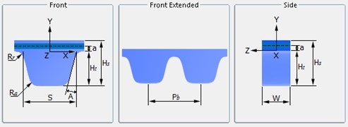
Fig. 3Synchronous belt parameter settings
a)
b)
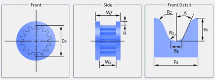
Table 1Nominal sizes of trapezoid teeth of type ZA and type ZB
Name | Pitch / mm | Angle / degree | Belt’ height / mm | Line difference /mm | Root fillet radius /mm | Tip radius / mm | Tooth height / mm | Tooth width / mm |
Code | 2 | |||||||
ZA | 9.525 | 40 | 4.1 | 0.686 | 0.51 | 0.51 | 1.91 | 4.65 |
ZB | 9.525 | 40 | 4.5 | 0.686 | 1.02 | 1.02 | 2.29 | 6.12 |
Table 2Synchronous pulley size
Name | Number of teeth | Gear width / mm | Rim height / mm | Outside diameter / mm | Root fillet radius / mm | Tip radius / mm | Tooth height / mm | Tooth width / mm |
Code | – | |||||||
Parameters | 20 | 76.2 | 7 | 199.08 | 2.69 | 2.82 | 10.29 | 11.61 |
Complete the assembly of the timing belt on the pulley, add the rotation pair between the driving wheel and the earth, the driven wheel and the earth, and apply the speed drive. Then click the Distance Sensor icon under the Sensor module in the Belt Kit to set the displacement sensor. After the completion of the effect as shown.
Fig. 4Synchronous pulley parameter setting
a)
b)
Fig. 5Synchronous belt simulation model
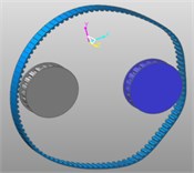
a)

b)
3.2. Model simulation
Dyn/Kin is called to simulate the model. Our initial simulation time is 5 seconds and the total number of steps is 100. Although the higher the number of simulation steps, the higher the accuracy of the simulation results [4], the longer the simulation takes. The simulation settings include the setting of the gravitational acceleration and the tension force. The direction of the gravitational acceleration is – direction, the size is 9806.65 mm/s2, and the tension force is set to 200 N-400 N. According to the set conditions, the system will calculate the model's displacement, velocity, acceleration, tension, and contact force.
Type ZA and ZB can be calculated using the following equation:
In the equation, – bandwidth, the unit is millimeters (mm). – Measuring force, the unit is Newton (N).
4. Simulation results and analysis
In the simulation animation, it can be seen that the speed of the synchronous belt suddenly increases under the driving of the driving wheel, and during the movement between the two pulleys, the timing belt vibrates, and a certain degree of sag occurs. After a period of operation, the belt and driven wheels operate at a constant speed to achieve a stable state.
It can be seen from the simulation animation that during the movement of the model, lateral vibration occurs in the synchronous belt, and the maximum value of the measured lateral pendulum momentum is about 0.221 mm, and the average value is 0.155 mm. The results of multiple measurements showed that there was not much difference from the above figure, and the error was within 0.1 mm, which fully met the requirements of measurement accuracy in national standards [5]. The time-dependent displacement curve of the belt along the direction in the coordinate system. The abscissa is time and the ordinate is displacement. As can be seen from the figure, the timing belt shifts periodically. After the start of the timing belt, after a small phase of movement, the descending segment in the direction visually indicates that the teeth have entered the meshing phase. The direction trough indicates that the timing belt reaches the leftmost end of the driving wheel, and the peak represents the rightmost position of the driven wheel. After a period of time, it re-enters the mesh and circulates in sequence.
From Figs. 6, 7, it can also be seen that the curve shows the lateral vibration characteristics when the timing belt reaches the meshing phase with the driven wheel after the first meshing of the timing belt and the disengaging of the driving wheel. Facts have proved that the turbulence along the direction is harmful, and the turbulence in this direction will lead to increased wear of the toothed teeth. If the belt speed is too high, a large amount of frictional heat will be generated, which will affect the use of the timing belt. Lifespan, so reducing the fluctuation in this direction will bring important significance to the drive. The movement situation reflected by the integrated displacement curve is in good agreement with the actual situation, and the simulation of the real situation can be achieved.
Fig. 6Displacement sensor results
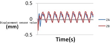
Fig. 7Synchronous belt displacement curve
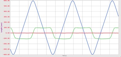
Fig. 8The speed curve of the timing belt in three directions
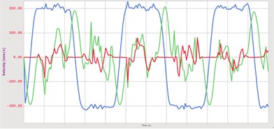
Fig. 9The initial tension is 480 N
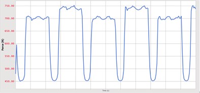
Fig. 10The initial tension is 540 N
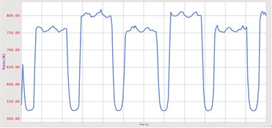
Fig. 6 and Fig. 7 are the changes of the speed of the belt in the three directions and the graphs of changes in the tension. As can be seen from the figure, there is a fluctuation phase in the speed of the timing belt. The timing belt maintains the pre-tightening force at a stage in which the timing belt does not engage with both pulleys, and shows a relatively stable pre-tension state. When the timing belt meshes with the pulley, it is subjected to the squeezing of the pulley teeth and the friction effect of the pulley on the belt teeth, and the tension force in the belt may change.
The resultant force changes curve of the contact force during the movement of the timing belt. As can be seen from the figure, the timing belt is not meshed with the driving wheel and the driven wheel before 0.3 seconds, so the contact force is zero. Corresponding to the other graphs, at the time of 0.3 seconds, the timing belt comes into contact with the driving wheel and enters the meshing stage, and the contact force begins to appear. Due to the inertial action, at the moment of contact, the timing belt will receive a large impact force. Under the action of this force, the toothed belt will momentarily be in a non-contact state or a small area contact state, and the belt will be instantly shortened. The other side of the belt will be in contact with the gear teeth, so it will produce contact force. The different contact areas of toothed and belted teeth, elastic sliding, material differences, and toothed errors cause the magnitude of contact force to fluctuate numerically.
Fig. 11Tension force variation curve of synchronous belt
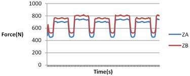
Fig. 12Synchronous belt contact force curve
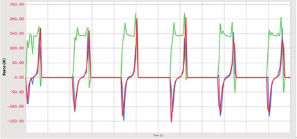
It is concluded that the contact force has a maximum value throughout the meshing process, and the magnitude of the specific value is related to the defined contact parameters. At 0.57 seconds, the timing belt meshes with the driving wheel and the contact force becomes zero. A certain moment in the -direction when the timing belt meshes is compared and analyzed, there is also a contact force, which is mainly due to the tooth-direction error of the timing belt and installation accuracy.
5. Conclusions
Using RecurDyn Software a belt movement model is established to fully understand the dynamic characteristics of the belt driving process, and the movement of the system can be conveniently and intuitively observed through the movement of the solid model. At the same time, the dynamic parameters of the system can be obtained, for example, the timing belt along the movement process. Three directions of displacement, speed, acceleration and other parameters. The displacement sensor can also measure the lateral vibration characteristics of any belt in any part of the synchronous belt, which provides a basis for the study of the lateral swing of the timing belt.
References
-
Shi Yaochen Research on Vibration and Noise of Vehicle Synchronous Belt Drive. Changchun University of Technology, 2016.
-
Guo Jianhua, Jiang Hongyuan, Meng Qingxin, et al. Experimental study on the noise and vibration of the new type of synchronous belt of herringbone teeth. Vibration and Impact, Vol. 34, Issues 17-120, 2015, p. 123-141.
-
Zhou Tao, Wei Menglin, Xiong Shengsheng, et al. Multibody dynamics simulation based on RecurDyn. CAD/CAM and Manufacturing Informatization, Vol. 8, 2004, p. 44-45.
-
Yang Demin Research on Multi-Joint Robot Dynamics Simulation Based on RecurDyn. Shanghai Normal University, 2016.
-
Vehicle Timing Belt GB12734-2003 National Quality Inspection Bureau, 2004.
Cited by
About this article

