Boundary condition identification of a clamped honeycomb sandwich panel based on thin-layer element

Xu, Yu; Cao, Zhifu; Jiang, Dong

doi:10.21595/jve.2019.20725

Journal of Vibroengineering

Browse Journal

Submit article

Published: 31 December 2019

Check for updates

Boundary condition identification of a clamped honeycomb sandwich panel based on thin-layer element

Yu Xu¹

Zhifu Cao²

Dong Jiang³

^{1, 2, 3}School of Mechanical and Electronic Engineering, Nanjing Forestry University, Nanjing, 210037, China

Corresponding Author:

Dong Jiang

Cite the article Download PDF

Downloads 1140

WoS Core Citations 1

CrossRef Citations 1

Abstract

The stiffness of boundary conditions in mechanical structures is difficult to represent. An approach on high fidelity modeling of the clamped boundary condition is proposed in this paper. Firstly, the normal and tangential stiffness of the contact surface of the clamped boundary condition is parameterized by using thin-layer element with isotropic material. Secondly, the material parameter is identified by minimizing the discrepancy between the calculated results and the experimental data, and parameter identification can be treated as an optimization problem. Experimental investigation is undertaken to verify the proposed method by employing an aluminum honeycomb panel, the numerical model of which is constructed by using the equivalent theory. Thin-layer elements with different properties are used to simulate the mechanical properties in different area of the boundary conditions, and the experimental modal data is adopted to identify the material parameters. Results show that the weighted matrix is a crucial option in the parameter identification procedure, and the width to thickness ratio of the thin layer element has a great influence on the identification results. After parameter identification, the error of the first three order of the modal frequencies is less than 2.7 %, the thin-layer element can accurately reflect the mechanical performance of clamped boundary condition.

1. Introduction

Structural dynamic performance is strongly affected by boundary conditions, which should be considered appropriately in both theoretical and numerical analysis. The effects of the boundary conditions on the performance of the mechanical structures are always underestimated and difficult to be determined [1]. The exist inappropriate methods for modeling of boundary stiffness, such as idealizing constraints into completely rigid and modelling ostensibly similar boundaries refer to the previous experiences, can be applied to characterize the boundary conditions in an oversimplified way, which will inevitably lead to errors in structural dynamics modeling.

Due to the crucial importance of mechanical behavior of boundary condition in engineering structures [2, 3], investigations on modeling of which have attracted interests of researchers [2-5]. The intuitive approach to determine the stiffness of clamped boundary conditions by using contact model between rough surfaces [6-8], Ahmadian and Zamani [9] studied the local nonlinear mechanism by experimentally observing the behavior of a beam structure with micro-slip/slap at the clamped end, these models can reflect the contact mechanism through analysis the asperities behavior of the real contact area, and the qualitative nonlinear contact stiffness can be derived. However, the contact analysis for boundary conditions will be very expensive in time consuming when apply in modeling of complex structures. Simplified equivalent modeling is the alternative method to represent the contact mechanics relationship and the boundary stiffness.

Identification of the boundary conditions from experimental data is an effective solution to improve the modeling accuracy. Pabst and Hagedorn [10] proposed an inverse method to identify the boundary stiffness and damping parameters of a visco-elastically clamped beam by using modal data, in which the boundary conditions was parametrized with a torsional spring-damper, and a translational spring-damper. Yang et al. [11] constructed a numerical model to solve multi-variables inverse problems for a beam with elastic boundary support, in which the static responses were employed and the elastic supports and constitutive parameters can be identified by using Levenberg-Marquardt algorithm. Wang [12] extended the cross-model cross-mode method for model updating by incorporating the connection flexibility and boundary conditions, the flexible joints and boundary conditions can be simultaneously updated. Yang et al. [13] proposed an approach using frequency response functions to identify the joint parameters including the rotational stiffness, which the accuracy of the identified results is strongly sensitive to the parameters. Baruh and Boka [14] modeled boundary conditions using axial and torsional springs, the orthogonality condition and the system eigenvectors were adopted to identify the spring constants. Boundary stiffness are simplified as spring models in the above researches, modeling difficulties will arise when apply spring models to complex structures, and the deficiency is obvious for modeling large contact surface.

Parameterization plays an important role in the stiffness identification of boundary conditions. Mottershead et al. [1] indicated that parameterization is critical in updating of boundary conditions, the boundary stiffness in a cantilever was modeled as the effective length of elements closest to the joint, but in some cases, the corrected matrices will lose connection to the physical significance while matching the experimental modal data. Noll et al. [15] inversely identified an elastic metal beam end-supported by elastomeric joints by revising non-diagonal terms in the stiffness matrix. The above stiffness characterization methods can be approximately parametrized the boundary stiffness, however, modeling complexities are still exit. In order to solve this problem, thin-layer element has been introduced to model the dynamics of mechanical joints [16-18], The concept of which was firstly proposed by Desai [19] who applied to the contact analysis in geotechnical engineering, and has been widely applied in equivalent modeling of joints, The normal and tangential stiffness of the contact surface can be accurately represented by the thin-layer elements.

Based on the basic theory of thin-layer element, this paper parameterized the contact surface of the clamped boundary. The elastic parameters of the thin-layer element are identified by using the experimental modal data. Besides, parameters such as the weight matrix used in the parameter identification, the width to thickness ration of the thin-layer element should be considered in the identification procedure, because of these parameters control the identification efficiency and the accuracy.

2. Basic theory

2.1. Thin-layer element

Thin-layer element is used to simulate the contact interface by defining a layer of elements. The size of thin-layer element is $l_{1} \times l_{2} \times d$ , according to the principle of virtual displacement, the virtual work of the element can be expressed as:

1

δ W = \int_{0}^{l_{1}} \int_{0}^{l_{2}} \int_{0}^{d} {\{σ\}}^{T} \{δ ε\} d x d y d z = δ {\{u\}}_{n o d a l}^{T} [K] {\{u\}}_{n o d a l},

in which $l_{1}$ and $l_{2}$ are the in-plane lengths of the thin-layer elements in the local coordinate system, and $d$ is the out-of-plane thickness. Fig. 1 shows isoparametric transformation of thin-layer element. Stiffness matrix [ $K$ ] of thin-layer element can be expressed as:

2

[K] = \int_{V_{e}} {[B]}^{T} [D] [B] d V = \int_{- 1}^{1} \int_{- 1}^{1} \int_{- 1}^{1} {[B]}^{T} [D] [B] d e t ([J]) d ξ d η d ζ,

where $ξ$ , $η$ , $ζ$ are natural coordinate symbols, [ $J$ ] is the Jacobian matrix, and when the coordinates of the natural and local coordinates are consistent, which can be written as:

3

[J] = [\begin{array}{l} \partial x / \partial ξ & \partial y / \partial ξ & \partial z / \partial ξ \\ \partial x / \partial η & \partial y / \partial η & \partial z / \partial η \\ \partial x / \partial ζ & \partial y / \partial ζ & \partial z / \partial ζ \end{array}] = [\begin{matrix} l_{1} / 2 & 0 & 0 \\ 0 & l_{2} / 2 & 0 \\ 0 & 0 & d / 2 \end{matrix}] .

By using of two-node Gaussian integration method, the following numerical expression for stiffness matrix [ $K$ ] of thin-layer element can be obtained:

4

[K] = \sum_{i = 1}^{2} \sum_{j = 1}^{2} \sum_{k = 1}^{2} {[B (ξ_{i}, η_{j}, ζ_{k})]}^{T} [C] [B (ξ_{i}, η_{j}, ζ_{k})] d e t ([J (ξ_{i}, η_{j}, ζ_{k})]) w_{ξ, i} w_{η, j} w_{ζ, k},

where $w_{ξ}$ , $w_{η}$ , and $w_{ζ}$ are the Gaussian integral weight function.

Fig. 1Isoparametric change of thin-layer element

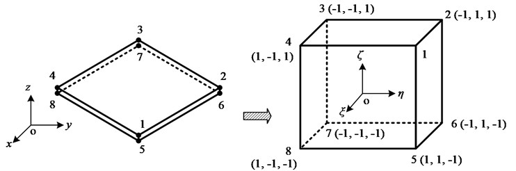
It is assumed that the thickness $d$ of the thin-layer element is much smaller than the feature sizes $l_{1}$ and $l_{2}$ . In this case, the in-plane strain components $(ε_{x}, ε_{y}, γ_{x y})$ and the stress components $(σ_{x}, σ_{y}, τ_{x y})$ of the element are ignored. $\partial N_{i} / \partial z$ is larger than $\partial N i / \partial x$ and $\partial N i / \partial y$ and can be analyzed by shape functions of element. Under this circumstances, $\partial N i / \partial x = \partial N i / \partial y \approx$ 0, which leads to the strain component $ε_{x} = ε_{y} = γ_{x y} \approx$ 0. Therefore, only three strain components at the Gaussian point of the thin-layer element are not zero. The strain component can be simplified to $ε = {[ε_{z} γ_{y z} γ_{z x}]}^{T}$ . The normal direction ( $n$ ) and two tangential direction ( $t$ ) of the contact surface are defined as the local coordinate system $(z, x, y)$ of thin-layer element. According to the previous analysis, assuming that the normal and tangential contact properties of the interface are independent and the two tangential contact properties are consistent. The constitutive equation of the thin-layer element that characterizes the contact properties of the interface is given by the following equation:

5

\{\begin{array}{l} σ_{n} \\ τ_{t x} \\ τ_{t y} \end{array}\} = [\begin{matrix} E_{n} & 0 & 0 \\ 0 & G_{t} & 0 \\ 0 & 0 & G_{t} \end{matrix}] \{\begin{array}{l} ε_{n} \\ γ_{t x} \\ γ_{t y} \end{array}\} .

$E_{n}$ and $G_{t}$ are the normal elastic modulus and tangential shear modulus, respectively, which are determined by the contact surface properties of the connecting structure. If the contact performance is coupled to the normal and tangent, then the coupling term can be added to the constitutive relationship Eq. (5). In the finite element analysis, the thin layer element integrated isotropic material can be used to simulate the contact interface, the constitutive relationship is expressed as:

6

\{\begin{array}{l} σ_{x x} \\ σ_{y y} \\ σ_{z z} \\ τ_{x y} \\ τ_{y z} \\ τ_{z x} \end{array}\} = [\begin{array}{l} λ + 2 G & λ & λ \\ λ + 2 G & λ \\ λ + 2 G \\ G \\ G \\ s y m & G \end{array}] \{\begin{array}{l} ε_{x x} \\ ε_{y y} \\ ε_{z z} \\ γ_{x y} \\ γ_{y z} \\ γ_{z x} \end{array}\},

7

λ = \frac{G (E - 2 G)}{E - 3 G} = \frac{E ν}{(1 + ν) (1 - 2 ν)},

in which $λ$ is lame constant, $G = E / 2 (1 + ν)$ is shear modulus. the isotropic material has only 2 independent material parameters. According to the basic theory of thin-layer element, the constitutive equation of the material will be degenerated to the following form:

8

\{\begin{matrix} σ_{z} \\ τ_{y z} \\ τ_{z x} \end{matrix}\} = [\begin{matrix} λ + 2 G & 0 & 0 \\ 0 & G & 0 \\ 0 & 0 & G \end{matrix}] \{\begin{matrix} ε_{z} \\ γ_{y z} \\ γ_{z x} \end{matrix}\} .

In this condition, the normal elastic constant and the tangent elastic constant are correlated.

The selection of different thickness of thin layer element will have a great influence on the calculation results. When the thickness is too large, the element has six strain components, and it is difficult to accurately reflect the mechanical characteristics of the contact interface. When the thickness is too small, the value of the determinant of Jacobian matrix approaches to zero, the matrix is ill conditioned and difficult to solve, and the displacement strain relation can’t be calculated by finite element method. A ratio coefficient is defined for the selection of thickness of a thin-layer element as follows:

9

R = \frac{m a x (l_{1}, l_{2})}{d} .

Desai et al. [20] recommended that $R$ should be selected in the range of 10-100.

The constitutive relation of the material can be integrated into the thin-layer element and the finite element dynamic analysis of the connection structure can be carried out. Vibration test data are used to identify the parameters of the thin-layer element. And the influence of weighted matrix and the ratio coefficient of thin-layer element $R$ on the identification results is researched.

2.2. Parameter identification

In this paper, material parameter identification of thin-layer elements is transformed into an optimization problem. The minimum value of the objective function is as follows:

10

\{\begin{array}{l} M i n J (p) = ε_{f}^{T} W ε_{f} = {‖W^{1 / 2} (z^{m} - z^{a} (p))‖}_{2}^{2}, \\ s . t . p_{1} \leq p \leq p_{2}, \end{array}

in which $ε_{f} = z^{m} － z^{a} (p)$ is the residual term represents the discrepancies between the experimental modal data and the calculated results, the modal data including the modal frequencies and mode shapes. $W$ is the weighted matrix, which reflects the relative weight of modal parameters. In general, $W$ is the identity matrix $I$ or [diag( $z^{m}$ )]^-2.

The real value of the elastic parameters is set to $p$ and the initial value is $P_{0}$ . The first order Taylor expansion of the eigenvalues $Λ$ and the mode matrix $ϕ$ at the $p_{0}$ point is as follows:

11

Λ (p) = Λ (p_{0}) + \overset{n}{\sum_{j = i}} \frac{\partial Λ}{\partial p_{j}} Δ p_{j} Φ (p) = Φ (p_{0}) + \overset{n}{\sum_{j = i}} \frac{\partial Φ}{\partial p_{j}} Δ p_{j},

where $p_{j}$ is the updating elastic parameters. When objective function is used for iterative solution, the problem of the $j$ th iterations is described as followed:

12

W^{(\frac{1}{2})} (z^{m} - z_{j}^{a}) = S_{j} Δ p_{j} = S_{j} (p_{j + 1} - p_{j}),

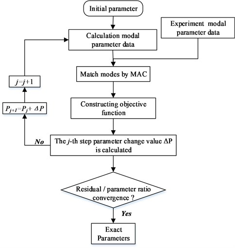
where $S_{j}$ represents the weighted Jacobian matrix of modal parameters to the updating parameters which is generally treated as the sensitivity matrix. $P_{j + 1}$ can be obtained by iterative solution of numerical analysis method until the identification parameter $p$ converges. At the same time, the calculation of modal parameters satisfies the requirement of precision. Finally, the accurate contact surface material parameters are obtained. The parameter identification procedure is shown as shown in Fig. 2.

Fig. 2The flow chat of parameter identification

3. Case studies: a clamped honeycomb panel

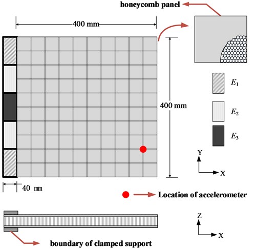
The one end clamped aluminum honeycomb sandwich panel which can be seen in Fig. 3, The contact surface is modeled by thin-layer elements of three different properties. The honeycomb sandwich panel is shown in Fig. 4, the dimensions is 400 mm×400 mm×16.3 mm. elastic Modulus $E_{s}$ is 68 GPa and density is 2700 kg/m³, Adhesive material is epoxy resin, the elastic Modulus $E_{s}$ is 5 GPa and density is 1500 kg/m³.

3.1. Equivalent modeling

The honeycomb core is generally considered to resist transverse shear deformation, neglecting lateral shearing stress, the honeycomb core is equivalent to an orthotropic material of uniform thickness and the same height as the honeycomb core. As a result, the honeycomb sandwich composite is a three-layer structure, an upper and a lower panels, and the middle is an equivalent core sandwich structure. Face sheet and the core layer are bonded through the adhesive layer, the mechanical property of the adhesive layer is worse than the panel and the core material. The interlaminar shear effect caused by the weak layer has an important influence on the macroscopic mechanical properties of the sandwich material. Therefore, the influence of the adhesive layer on the dynamic characteristics of the honeycomb sandwich composite can’t be neglected. Fig. 5 shows the finite element model of honeycomb plate.

Fig. 3The experimental arrangement of the clamped honeycomb panel

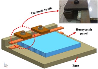
Fig. 4The geometry of honeycomb sandwich panel

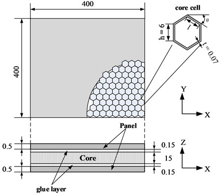
The honeycomb sandwich panel is modeled using the equivalent method. Shear deformation, axial tension and compression deformation analysis equivalent elastic parameters are ignored. The cell wall of the core is simplified as a planar Euler-Bernoulli beam. The equivalent elastic parameters in the $x$ - $y$ plane can be obtained. In particular, the unit cell of honeycomb core is a regular hexagon that the $l = h$ , $θ =$ 30°. the in-plane elastic parameters of the core are expressed as:

13

E_{c x} = E_{c y} = \frac{4}{\sqrt{3}} {(\frac{t}{l})}^{3} E_{s},

14

G_{c x y} = \frac{\sqrt{3} γ}{2} {(\frac{t}{l})}^{3} E_{s},

where $E_{c x}$ and $E_{c y}$ are the equivalent elastic modulus, $G_{c x y}$ is equivalent shear modulus, $E_{s}$ is elastic modulus of honeycomb core material. Elastic modulus $E_{c z}$ in the z direction can be got by tension and compression stiffness equivalent:

15

E_{c z} = \frac{2}{\sqrt{3}} \frac{t}{l} E_{s} .

Equivalent material parameters which core equivalent shear modulus $G_{c x z}$ and $G_{c y z}$ have the most impact on the dynamic performance of the equivalent model. The stress distribution is complicated When the honeycomb core considers the pure shear of three planes. The minimum potential energy principle and the principle of the minimum residual energy can be used to estimate the range of the two out-of-plane shear modulus:

16

G_{c x z} = \frac{γ}{\sqrt{3}} \frac{t}{l} G_{s},

17

G_{c y z} = \frac{\sqrt{3} γ}{2} \frac{t}{l} G_{s},

where $G_{s}$ in the formula is the shear modulus of the honeycomb core material; $γ$ is the updating factor, which theoretical value is equal to 1, generally take 0.4-0.6 in engineering applications. As the following formula, the equivalent density of honeycomb core can be obtained by mass equivalent:

18

ρ_{e q} = \frac{8}{3 \sqrt{3}} \frac{t}{l} ρ_{s} .

In summary, aluminum honeycomb sandwich panel and glue layer are constructed as an laminate. Orthotropic honeycomb core layers are modeled using solid elements. Clamped boundary contact layer is modeled by isotropic thin-layer elements. The finite element model’s boundary conditions are achieved by constraining six degrees of freedom.

Fig. 5FEM of honeycomb plate

3.2. Parameter identification

3.2.1. Weight matrices

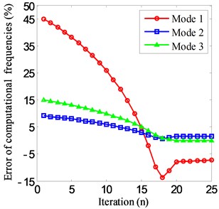
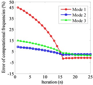
The influence of different weighting matrices on the results of parameter identification is studied by establishing a thin-layer element with $R =$ 100. The frequency convergent curves when weighted matrices are identity matrix and [diag( $z^{m}$ )]^-2 are shown in Fig. 6, Table 1 is the results comparison of natural parameter identification.

Table 1Wε=I Comparison of natural frequency

Mode	$f^{m}$ /Hz	Initial		$W_{ε} = I$		$W_{ε} = {[d i a g (z^{m})]}^{- 2}$
Mode	$f^{m}$ /Hz	$f^{a}$ /Hz	Error (%)	$f^{a}$ /Hz	Error (%)	$f^{a}$ /Hz	Error (%)
1	49.59	71.94	45.07	47.13	–4.96	49.27	–0.64
2	199.8	218.09	9.15	203.84	2.03	205.05	2.63
3	411.93	473.83	15.3	412.04	0.03	416.16	1.03

Fig. 6Frequency iteration convergence curve: a) Wε=I; (b) Wε=diagzm-2

a)

b)

After the identification, the accuracy of the inherent frequency is greatly improved. The error of the first three order calculation natural frequency is less than 2.63 %, when [diag( $z^{m}$ )]^-2 is selected as the weighted matrix $W_{ε}$ .

3.2.2. Width to thickness ratio

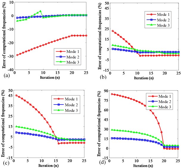
Based on the above results, the weighted matrix is determined as $W_{ε} = {[d i a g (z^{m})]}^{- 2}$ . Then researches of parameter identification are carried out when the $R$ of thin layer elements is 10, 50, 100, 500, respectively.

Frequency iteration convergence curve under different $R$ is shown in Fig. 7. The convergence error is reduced with the increase of the width and thickness ratio. However, more iterations are need for convergence.

Table 2Comparisons of calculated frequency errors under different R

Mode	$f^{m}$ /Hz	$R =$ 10		$R =$ 50		$R =$ 100		$R =$ 500
Mode	$f^{m}$ /Hz	$f^{a}$ /Hz	Error (%)	$f^{a}$ /Hz	Error (%)	$f^{a}$ /Hz	Error (%)	$f^{a}$ /Hz	Error (%)
1	49.59	42.53	–14.23	49.30	–0.56	49.27	–0.64	49.32	–0.54
2	199.8	200.53	0.36	205.10	2.65	205.05	2.63	205.14	2.67
3	411.93	414.37	0.59	414.70	0.68	416.16	1.03	414.47	0.62

Table 2 is the comparison of calculation natural frequency and parameter identification results of thin-layer element under different $R$ . In this case, the $R$ is increased by changing the direction of the thickness. The stiffness properties of the contact surface are determined by the elastic parameters and the thickness of the thin layer element. The ratio coefficient $R$ of the thin layer element has a great influence on the identification results. The error of convergence result is improved with the increase of $R$ but more iterations are needed.

Fig. 7Frequency iteration convergence curve under different R: a) R= 10; b) R= 50; c) R= 100; d) R= 500

4. Conclusions

An approach on identifying the stiffness of the contact surface of the clamped boundary condition is proposed in this paper. The contact surface is modeled based on the theory of thin-layer element, and modal parameters are used to identify the material parameters of thin-layer element which represents the stiffness of the contact surface. The equivalent modeling method are employed to establish the simulation model of aluminum honeycomb panel. Three kinds of thin layer elements with different properties are used to simulate the mechanical change of the boundary. The effect of the weighted matrix and the proportion of $R$ on the convergence results are discussed. It is concluded that the convergence error of the parameter can be reduced effectively when weighted matrix is [diag( $z^{m}$ )]^-2.

References

Mottershead J. E., Friswell M. I., Ng G. H. T., et al. Geometric parameters for finite element model updating of joints and constraints. Mechanical Systems and Signal Processing, Vol. 10, Issue 2, 1996, p. 171-182.

Publisher
Demir C., Izmirli S. B. The effects of support size on the vibration of the point supported plate. International Journal of Physical Sciences, Vol. 6, Issue 8, 2011, p. 1920-1928.

Search CrossRef
Friswell M. I., Wang D. The minimum support stiffness required to raise the fundamental natural frequency of plate structures. Journal of Sound and Vibration, Vol. 301, Issues 3-5, 2007, p. 665-677.

Publisher
Ritto T. G., Sampaio R., Aguiar R. R. Uncertain boundary condition Bayesian identification from experimental data: A case study on a cantilever beam. Mechanical Systems and Signal Processing, Vol. 68, Issue 69, 2016, p. 176-188.

Publisher
Pietrzyk M., Madej L., Rauch L., et al. Identification of material models and boundary conditions. Computational Materials Engineering, Achieving High Accuracy and Efficiency in Metals Processing Simulations, 2015, p. 153-208, https://doi.org/10.1016/B978-0-12-416707-0.00004-1.

Publisher
Goedecke A., Jackson R. L., Mock R. A fractal expansion of a three dimensional elastic-plastic multi-scale rough surface contact model. Tribology International, Vol. 59, 2013, p. 230-239.

Publisher
Belghith S., Mezlini S., Belhadjsalah H., et al. Modeling of contact between rough surfaces using homogenisation technique. Comptes Rendus Mecanique, Vol. 338, Issue 1, 2010, p. 48-61.

Publisher
Pei L., Hyun S., Molinari J., et al. Finite element modeling of elasto-plastic contact between rough surfaces. Journal of the Mechanics and Physics of Solids, Vol. 53, Issue 11, 2005, p. 2385-2409.

Publisher
Ahmadian H., Zamani A. Identification of nonlinear boundary effects using nonlinear normal modes. Mechanical Systems and Signal Processing, Vol. 23, Issue 6, 2009, p. 2008-2018.

Publisher
Pabst U., Hagedorn P. Identification of boundary conditions as a part of model correction. Journal of Sound and Vibration, Vol. 182, Issue 4, 1995, p. 565-575.

Publisher
Yang H. T., Yang B., Li H. T. Numerical solution of multi-variables inverse problem for a beam with elastic boundary supports. Dalian Ligong Daxue Xuebao/Journal of Dalian University of Technology, Vol. 51, Issue 4, 2011, p. 469-472, (in Chinese).

Search CrossRef
Wang S. Model updating and parameters estimation incorporating flexible joints and boundary conditions. Inverse Problems in Science and Engineering, Vol. 22, Issue 5, 2013, p. 727-745.

Publisher
Yang T. C., Fan S. H., Lin C. S. Joint stiffness identification using FRF measurements. Computers & Structures, Vol. 81, Issues 28-29, 2003, p. 2549-2556.

Publisher
Baruh H., Boka J. B. Modeling and identification of boundary conditions in flexible structures. International Journal of Analytical and Experimental Modal Analysis, Vol. 8, 1993, p. 107-117.

Search CrossRef
Noll S., Dreyer J. T., Singh R. Identification of dynamic stiffness matrices of elastomeric joints using direct and inverse methods. Mechanical Systems and Signal Processing, Vol. 39, Issues 1-2, 2013, p. 227-244.

Publisher
Schmidt A., Bograd S., Gaul L. Measurement of join patch properties and their integration into finite-element calculations of assembled structures. Shock and Vibration, Vol. 19, Issue 5, 2012, p. 1125-1133.

Publisher
Jalali H., Hedayati A. Ahmadian H. Modelling mechanical interfaces experiencing micro-slip/slap. Inverse Problems in Science and Engineering, Vol. 19, Issue 6, 2011, p. 751-764.

Publisher
Bograd S., Reuss P., Schmidt A., et al. Modeling the dynamics of mechanical joints. Mechanical Systems and Signal Processing, Vol. 25, Issue 8, 2011, p. 2801-2826.

Publisher
Desai C. S., Zaman M. M., Lightner J. G., et al. Thin-layer element for interfaces and joints. International Journal for Numerical and Analytical Methods in Geomechanics, Vol. 8, Issue 1, 1984, p. 19-43.

Publisher
Sharma K. G., Desai C. S. Analysis and implementation of thin-layer element for interfaces and joints. Journal of Engineering Mechanics, Vol. 118, Issue 12, 1992, p. 2442-2462.

Publisher

Cited by

Identification of Pre-Tightening Torque Dependent Parameters for Empirical Modeling of Bolted Joints

Yu Tian | Hui Qian | Zhifu Cao | Dahai Zhang | Dong Jiang

(2021)

About this article

Received

15 April 2019

Accepted

26 October 2019

Published

31 December 2019

SUBJECTS

Dynamics of smart and functionally graded materials

DOI

https://doi.org/10.21595/jve.2019.20725

Keywords

boundary conditions

honeycomb panel

thin-layer element

stiffness identification

modal data

This is an open access article distributed under the Creative Commons Attribution License, which permits unrestricted use, distribution, and reproduction in any medium, provided the original work is properly cited.

Previous article in issue Previous

Research article

2022 06 30

Multi-objective structural optimization of honeycomb cells

Xu Zhang, Zhaoming Su, Wei Li, Xuejuan Niu, Zituo Wang

Research article

2019 04 25

Modal analysis of sandwich panel with composite laminated faces

Eva Kormanikova

Research article

2018 08 15

A unified Gram-Schmidt-Ritz formulation for vibration and active flutter control analysis of honeycomb sandwich plate with general elastic support

Huagang Lin, Dengqing Cao

Research article

2018 06 30

On the selection of boundary conditions for top tensioned risers facing wave induced vibrations

Zohreh Sadat Haghayeghi, Mohammad Javad Ketabdari

Y. Xu, Z. Cao, and D. Jiang, “Boundary condition identification of a clamped honeycomb sandwich panel based on thin-layer element,” Journal of Vibroengineering, Vol. 21, No. 8, pp. 2286–2295, Dec. 2019, https://doi.org/10.21595/jve.2019.20725

Copy Extrica

Copied to clipboard!

TY  - JOUR
DO  - 10.21595/jve.2019.20725
UR  - https://doi.org/10.21595/jve.2019.20725
TI  - Boundary condition identification of a clamped honeycomb sandwich panel based on thin-layer element
T2  - Journal of Vibroengineering
AU  - Jiang, Dong
AU  - Xu, Yu
AU  - Cao, Zhifu
PY  - 2019
DA  - 2019/12/31
PB  - JVE International Ltd.
SP  - 2286-2295
IS  - 8
VL  - 21
SN  - 1392-8716
SN  - 2538-8460
ER  - 

Copy Ris

Copied to clipboard!

@article{Jiang_2019,
	doi = {10.21595/jve.2019.20725},
	url = {https://doi.org/10.21595/jve.2019.20725},
	year = 2019,
	month = {dec},
	publisher = {{JVE} International Ltd.},
	volume = {21},
	number = {8},
	pages = {2286--2295},
	author = {Dong Jiang and Yu Xu and Zhifu Cao},
	title = {Boundary condition identification of a clamped honeycomb sandwich panel based on thin-layer element},
	journal = {Journal of Vibroengineering}
}

Copy Bibtex

Copied to clipboard!

[1]D. Jiang, Y. Xu, and Z. Cao, “Boundary condition identification of a clamped honeycomb sandwich panel based on thin-layer element,” Journal of Vibroengineering, vol. 21, no. 8, pp. 2286–2295, Dec. 2019, doi: 10.21595/jve.2019.20725.

Copy IEEE

Copied to clipboard!

Jiang, Dong, Yu Xu, and Zhifu Cao. “Boundary Condition Identification of a Clamped Honeycomb Sandwich Panel Based on Thin-Layer Element.” Journal of Vibroengineering 21, no. 8 (December 31, 2019): 2286–95. https://doi.org/10.21595/jve.2019.20725.

Copy Chicago

Copied to clipboard!

Boundary condition identification of a clamped honeycomb sandwich panel based on thin-layer element

Abstract

1. Introduction

2. Basic theory

2.1. Thin-layer element

2.2. Parameter identification

3. Case studies: a clamped honeycomb panel

3.1. Equivalent modeling

3.2. Parameter identification

3.2.1. Weight matrices

3.2.2. Width to thickness ratio

4. Conclusions

References

Cited by

About this article

Related Articles