Abstract
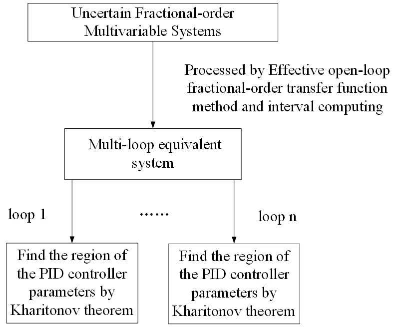
In this paper, a graphical tuning method for controllers parameters based on the open-loop fractional transfer function (FO-EOTF) method is proposed for fractional-order parameter uncertain multivariable system. The FO-EOTF method is proposed to transform the parameter uncertain fractional-order multivariable system into a set of independent parameter uncertain fractional-order univariate systems and determine the parameters regions of the univariate systems. The gain phase margin tester is used to further guarantee the robust performance of the controlled system. Finally, simulation result from the numerical simulation is presented to demonstrate the effectiveness of this method.
Highlights
- This paper mainly introduces a controller design method for uncertain fractional-order multi-variable systems
- Graphical value interval is beneficial to the selection of controller parameters
- The introduction of interval calculation can solve the impact of uncertainty on the system
1. Introduction
The industrial processes are often modeled by multivariate models. Fractional-order transfer function is always used to describe the industrial processes to improve the accuracy of multivariate system modeling. The parameters of models are usually uncertain due to the existence of measurement errors, machine aging and many other problems. Considering every input in the multivariable model may have impacts on outputs, the controller design of the multivariable model becomes very complex. Therefore, it is not feasible to treat the multivariable model as multiple univariate models directly. Meanwhile, the complexity of controller design for multivariable model will increase when the subsystems are fractional-order and the parameters of the multivariable system are uncertain. Multivariable system is confronted with decoupled issue when we design robust controller.
In past decades, many decoupling methods for the multivariable systems have been proposed. In literature [1], the SLC method is proposed to design the controllers of the multivariable system one by one in a certain matrix. Unfortunately, this method is very strict on the setting order of the controller. Li has proposed the practical multivariable control based on inverted decoupling and decentralized ADRC [2]. The modeling uncertainties, that significantly affect the robustness of the inverted decoupling control approach, are treated by ADRC outside of the decoupling structure. Jobrun has proposed a method for MIMO processes based on the multi-scale control scheme. The method tuning the controller parameters with the balanced sensitivity function [3, 4]. However, this method cannot be applied directly to the parameters uncertain multivariable system, because the uncertain parameters will bring huge calculation pressure to decoupling. There are also many optimization algorithms that can turn the parameter of controllers [5-7]. However, when the parameter of the system are uncertain, these algorithms will not be able to calculate the controller parameters. Therefore, a simplified decoupling method is needed to settle the coupling problem. The concept of an effective open-loop transfer function (EOTF) has been introduced and studied to design the controllers for multivariable systems by several researchers [8-13]. The core idea is to transform the multivariable system into a set of independent univariate systems. This method simplified the design of the controller while solving the coupling problem of the multivariable system. Vu [12] has proposed a method to design the controller and showed favorable control performance for multivariable system based on EOTF method and later studied by Jin [13].
Compared with integer-order calculus, the use of fractional calculus can be more accurate description of complex dynamic systems. For the fractional-order characteristic polynomials with time delay terms, the characteristic polynomial of fractional-order delay system is not a standard characteristic polynomial because of the existence of delay term and fractional order, while a quasi-characteristic polynomial that composed of the fractional power of the complex variable s and the delay term . Therefore, the algebraic methods such as Routh-Hurwitz method, which is already used to test the stability of integer order linear control systems, cannot be directly applied to the stability criterion of fractional delay control systems. Of course, since the characteristic polynomial is a function of complex variables, the stability test principle of the existing integer order-delay system can be applied. The Kharitonov theorem has been proposed and studied to replace the parameter uncertain univariate system via multiple boundary equations for integer order linear control systems [14-17]. For each boundary equation, the region of the controller parameters satisfying certain robustness and stability can be determined. The intersection of all regions obtained by boundary equations is the controller parameter interval of the parameter uncertain univariate system. For fractional-order systems, Hamamci [18] proposed a method to find the stable region of fractional-order PID controller. Hamamci extended the D-factorization method for fractional-order PID controller to fractional-order domain and obtained the stable region of fractional PID. Using the existing stability theory of fractional calculus equation and Kharitonov boundary theory, Petráš et al. [19] proposed an algebraic method to test the stability of fractional linear system with uncertainties. Gao et al. [20] studied the relative stability of fractional-order systems and obtained the stable region of fractional-order PID controller. However, none of the above methods directly consider the uncertainty of the model parameters of the controlled object. Due to the working condition of the servo drive system, the model parameters also change with the system state. Therefore, the graphical tuning method should be based on the uncertain parameter model, otherwise, the set controller parameters will not meet the strong robustness requirements of the servo drive system, thus affecting the control accuracy. In response to this problem, Zheng et al. [21] proposed a graphical tuning method of fractional order proportional integral derivative (FOPID) controllers for fractional order uncertain system achieving robust D-stability. Hajiloo et al. [22] calculates the value range of the FOPID controller by multi-objective optimization. At the same time, Saidi et al. [23] gives the tuning method of the FOPID controller for fractional order uncertain system from the frequency domain. However, these methods are only for univariate systems.
In this paper, a new method is proposed to determine the robustness stable region of the parameter uncertain fractional-order multivariable system based on the EOTF method and Kharitonov method. In particular, the proposed FO-EOTF method is used to transform the parameter uncertain multivariable system into a set of independent parameter uncertain univariate systems. Then, the independent parameter uncertain univariate systems is numerical implementation by Oustaloup algorithm. Finally, the Kharitonov method is introduced to determine the robustness stable region of the parameter uncertain univariate system.
2. Effective open-loop fractional-order transfer function
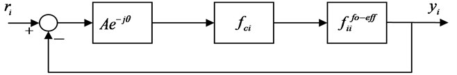
The entire closed-loop of the system is shown in Fig. 1, where , and are the inputs, internal variables and outputs, respectively. is the PID controller. is the parameter uncertain fractional-order multivariable system. The model is shown as follow:
Fig. 1Closed-loop of the parameter uncertain fractional-order multivariable system
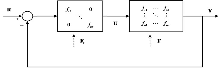
The parameters in model are uncertain in a certain interval. The general expression is:
where and are the numerator terms and denominator terms of the transfer function . and are the fractional-orders of numerator terms and denominator terms. and are the coefficients of numerator terms and denominator terms, respectively, which satisfy and . is the time delays term of which satisfies .
Fig. 2The concept of the FO-EOTF
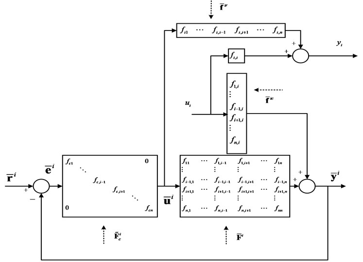
The FO-EOTF method mainly utilizes the self-stabilizing ability of the system to solve the coupling problem, thereby reducing the difficulty of the coupling problem for the controller design. The FO-EOTF of loop is defined as the transfer function relating with where loop is open while all other loops are closed, as shown in Fig. 2, where , and are the input, internal variable and output of loop , respectively. is the remaining parts of without . and are the column and row of without , respectively. is the remaining parts of without column and row . , and are the remaining parts of , and without , and .
When , can be written as:
Eq. (3) can be simplified as:
From Fig. 2, it is clear that is related to and . The corresponding relationship can be written as:
When the frequency is below the cut-off frequency [10], the relationship between and is:
Eq. (5) can be written as:
Fig. 3The closed-loop of multivariable system after FO-EOTF
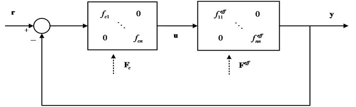
The influences from the controllers of the other loops are eliminated when tuning the controller of loop . Each loop can be obtained by Eq. (7). Thus, the entire multivariable system can be equivalent to a diagonal matrix system , which is:
From Fig. 3, we can know that the structure of the whole closed-loop control loop after replacing the parameter uncertain multivariable system with the parameter uncertain equivalent model . The equivalent model can effectively reduce the interference caused by the coupling factors between the systems, and also greatly reduce the amount of computation. The equivalent transfer function of loop in is only related to all elements in the system in Eq. (7). Assuming the general expression as:
where is consisted of and in Eq.(2), is consisted of . Similarly, the FO-EOTF model similar to Eq. (9) can be obtained for each parameter uncertain multivariable system. However, the general expression of in Eq. (9) is inconvenient to analyze and calculate because of the excessive time delay. Thus, Eq. (9) can be simplified as:
where , , , and are all uncertain in a certain interval. In literature [9], it is pointed out that when the numerator and denominator coefficients of the transfer function are fixed, the larger the delay term is, the smaller the stability domain. First, considering the parameters of non-time delay term in are fixed, the time delays are uncertain in a certain interval. Meanwhile, the coupling relationships among the coefficients of the time delays are ignored. Then, the coefficients of the time delays in molecular term take the maximum value . On the contrary, coefficients of the time delays in denominator term take the maximum value . Then, find the maximum values of and , that are and , and extract them out. Finally, the remaining parts after extraction are approximated by Taylor expansion. Take the 2×2 parameter uncertain system as an example:
where , and . Through Eq. (7), the FO-EOTF of loop 1 can be written as:
where:
Under the premise of ignoring the coupling relation of the time delay, the fluctuation interval of the time delay can be obtained, that are , and .
Find out , and according to the rules mentioned above. Then, and can be obtained by comparison. For the convenience of display here, assuming , that means . Then, the remaining part of the extract is processed by Taylor expansion. Thus, Eq. (12) can be rewritten as:
In Eq. (13), the coefficient of the time delay is fixed, and the other coefficients are uncertain values in certain intervals. Due to the infinite dimensional properties of fractional-order operators, it cannot be directly numerically implemented. In this paper, the Oustaloup algorithm is used to approximate it by continuous transfer function. When using the Oustaloup algorithm to approximate fractional-order operator, the approximating frequency band and the order of the approximated transfer function need to select at first. Here, the approximating frequency band is assumed and the approximating order is . The general transfer function of Oustaloup algorithm is expressed as:
where:
Therefore, Eq. (10) can be approximated by Oustaloup algorithm, which shown in Eq. (15) as:
3. Kharitonov theorem
It can be seen from Fig. 3, a multivariable system can be equivalent to multiple single variable systems after equivalent transformation. For general parameter uncertain univariate system, the corresponding boundary system can be obtained directly based on Kharitonov theorem. Then, the region of the controller parameters satisfying certain robustness for the parameter uncertain univariate system can be calculated. However, the premise of using the Kharitonov theorem is that the parameters of the uncertain model are linearly independent. The parameters and of the above FO-EOTF are determined by the coefficients in , showing a linear correlation. In order to simplify the calculation, ignore the coupling between the parameters, readjust the intervals of the parameters as and .
The controller used in this paper is PID controller. Taking loop as an example, the expression of the controller is:
where , and are the proportions, integrals and differential terms of controller , respectively. In order to satisfy the stability and certain robustness, a gain phase margin tester is added to the loop , as shown in Fig. 4. Thus, the characteristic polynomial of the loop can be obtained:
Fig. 4The closed-loop of multivariable system with gain phase margin tester
Substituting Eqs. (15) and (16) into Eq. (17), we get:
Eq. (18) can be written as:
Further algebraic manipulation of Eq. (19) results as:
where and are the real and imaginary parts of in respectively, while and are uncertain but bounded. Thus, Eq. (19) can be rewritten as:
When Eq. (21) satisfies the Hurwitz stability, the entire uncertain system satisfies the stability condition. In order to further simplify the computation, the Kharitonov theorem is used to deal with the Eq. (21). The theorem indicates that Eq. (21) can be replaced by a set of boundary equations:
For each boundary equation , there is a set of controllers that can make it stable. The intersection of controller parameters regions corresponding to each boundary equation is the final region of the controller parameters of the loop , that is . Due to the existence of the gain phase margin tester , the controller can make the equivalent open-loop transfer function stable while satisfying certain robustness.
Let , the Eqs. (22)-(29) can be written as:
where and are the real and imaginary parts of , respectively. Let and equal to zero:
where , , , , and are the remaining parts after the common factor is extracted. Using the Cramer rule, the equations about and can be obtained:
When the parameters in the right part of Eqs. (33) and (34) are fixed, a boundary line can be calculated in the plane. The controller parameters corresponding to the point in this line can make the system in Fig.4 critical stable. Then, it is necessary to determine the regions of the controllers parameters by using the Jacobian matrix of Eqs. (33) and (34). The Jacobian matrix are:
When , the left of the stable line facing the direction in which increases is the stable regions. When , the right of the stable line facing the direction in which increases is the stable regions. In this way, the stability interval for each boundary equation can be determined. Thus, the final stable range can be easily obtained.
4. Simulation
Assuming the model in Fig. 1 is a 2×2 parameter uncertain fractional-order multivariable:
where [0.9, 1], [0.8, 0.9], [1, 1.1], [0.9, 1.1], [1.7, 1.9], [1.9, 2], [1.5, 1.6], [1.6, 1.7], [0.45, 0.5], [0.4, 0.45], [0.25, 0.3] and [0.2, 0.25]. Assuming the loops need to satisfy the conditions of 8 dB and 30°. The final robust stable region of the loops can be calculated, as shown in Figs. 5-6.
Fig. 5Robust stable boundary lines of Δ1
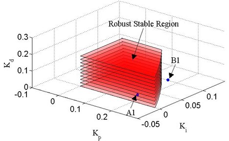
Fig. 6Robust stable boundary lines of Δ2
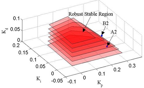
Fig. 7Responses of controllers A1 and A2
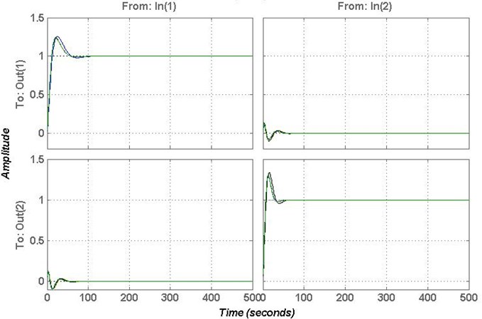
Three sets of controllers are selected (0.2, 0.01, 0.03), (0.2, 0.08, 0.04), (1, 0.5, 0.1), (0.25, 0.02, 0.03), ( 0.25, 0.05, 0.06) and (0.5, 0.5, 0.05) to verify the effectiveness of this method. Where, and are in robust stable region, and are in the stable region but outside of the robust stable region, and are outside the stable region. The responses of controllers and are shown in Fig. 7. The responses of controllers and are shown in Fig. 8. The responses of controllers and are shown in Fig. 9.
Fig. 8Responses of controllers B1 and B2
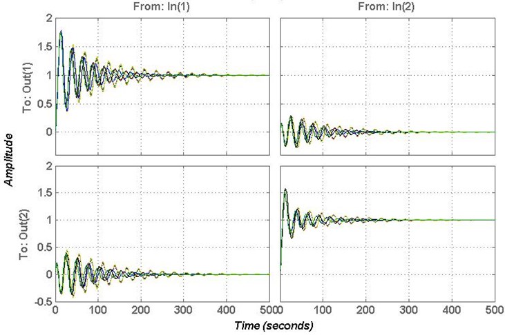
Fig. 9Responses of controllers C1 and C2
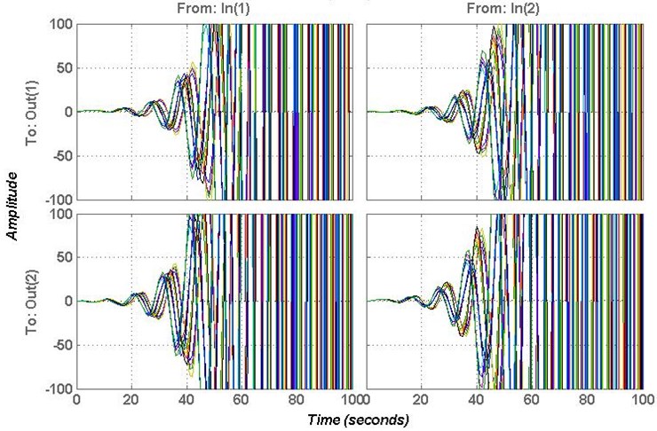
From Figs. 7-9, it clear that the controllers , , and can stable the system, but the controllers and cannot stable the system. In order to verify the effectiveness of the proposed method, the gain and phase margins of the controllers , , and are calculated to verify the robustness.
Fig. 10Bode plot of the controller A1 and A2
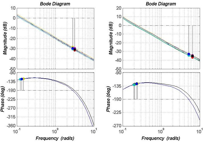
Fig. 11Bode plot of the controller B1 and B2
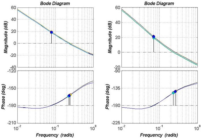
Fig. 10 shows the gain and phase margins of controller and . The gain margin of controller is in 28.7-31.6 dB, the phase margin is around 58 deg. The gain margin of controller is in 32.9-36.7 dB, and the phase margin is around 51 deg. Fig. 11 shows the gain and phase margins of controller and . The gain margin of controller is around –18.4 dB, the phase margin is in 15.9-18.2 deg. The gain margin of controller is around –21 dB, and the phase margin is in 32.5-37.1deg, which does not meet the limited conditions. Therefore, the controller in the robust stability region can make the system satisfy robustness.
5. Conclusions
In this paper, a unique graphical method are used to design the PID controller of the parameter uncertain fractional-order multivariable system. FO-EOTF is used to decouple multivariable systems and transform the multivariable system into a set of independent univariate systems. Based on Kharitonov theorem, a set of boundary systems is used to replace parametric uncertain fractional-order univariate systems. Then, the region of the PID controller parameters can be determined. In order to consider the robustness of the system, the gain phase margin tester is introduced. From the example, it can be seen that the proposed method can calculate the region of the PID controller parameters of the parameter uncertain fractional-order multivariable system. The parameters in the robust stable region can stabilize the system and meet certain robustness requirements. The parameters of the controller outside the robust stable region do not meet the requirements. The unique graphical approach helps to better understand how to determine the area of controller parameters.
References
-
Hovd M., Skogestad S. Sequential design of decentralized controllers. Automatica, Vol. 30, Issue 10, 1994, p. 1601-1607.
-
Li S., Junyi D., Donghai L., et al. A practical multivariable control approach based on inverted decouplingand decentralized active disturbance rejection control. Industrial and Engineering Chemistry Research, Vol. 55, Issue 7, 2016, p. 847-866.
-
Nandong J., Zang Z. Multi-loop design of multi-scale controllers for multivariable processes. Journal of Process Control, Vol. 24, Issue 5, 2014, p. 600-612.
-
Nandong J. Heuristic-based multi-scale control method of simultaneous multi-loop PID tuning for multivariable processes. Journal of Process Control, Vol. 35, 2015, p. 101-112.
-
Deng W., Yao R., Zhao H., et al. A novel intelligent diagnosis method using optimal LS-SVM with improved PSO algorithm. Soft Computing, Vol. 23, Issue 7, 2019, p. 2445-2462.
-
Deng W., Zhao H., Zou L., et al. A novel collaborative optimization algorithm in solving complex optimization problems. Soft Computing, Vol. 21, Issue 15, 2017, p. 4387-4398.
-
Deng W., Zhao H., Yang X., et al. Study on an improved adaptive PSO algorithm for solving multi-objective gate assignment. Applied Soft Computing, Vol. 59, 2017, p. 288-302.
-
Xiong Q., Cai W. J. Effective transfer function method for decentralized control system design of multi-input multi-output processes. Journal of Process Control, Vol. 16, Issue 8, 2006, p. 773-784.
-
Luan X., Chen Q., Liu F. Equivalent transfer function based multi-loop PI control for high dimensional multivariable systems. International Journal of Control, Automation and Systems, Vol. 13, Issue 2, 2015, p. 346-352.
-
Huang H. P., Jeng J. C., Chiang C. H., et al. A direct method for multi-loop PI/PID controller design. Journal of Process Control, Vol. 13, Issue 8, 2003, p. 769-786.
-
He M. J., Cai W. J., Wu B. F., et al. Simple decentralized PID controller design method based on dynamic relative interaction analysis. Industrial and Engineering Chemistry Research, Vol. 44, Issue 22, 2005, p. 8334-8344.
-
Nguyen T., Vu L., Lee M. Independent design of multi-loop PI/PID controllers for interacting multivariable process. Journal of Process Control, Vol. 20, Issue 8, 2010, p. 922-933.
-
Jin Q. B., Hao F., Wang Q. A multivariable IMC-PID method for non-square large time delay systems using NPSO algorithm. Journal of Process Control, Vol. 23, Issue 5, 2013, p. 649-663.
-
Kharitonov V. L. The asymptotic stability of the equilibrium state of a family of systems of linear differential equations. Differential Equations, Vol. 11, 1978, p. 2086-2088.
-
Pisano A., Caponetto R. Stability margins and H∞ co‐design with fractional-order PIλ controllers. Asian Journal of Control, Vol. 15, Issue 3, 2013, p. 691-697.
-
Yuanjay W. Determination of all feasible robust PID controllers for open-loop unstable plus time delay processes with gain margin and phase margin specifications. ISA Transactions, Vol. 53, Issue 2, 2014, p. 628-646.
-
Fang B. Design of PID controllers for interval plants with time delay. Industrial Control Computer, Vol. 24, Issue 10, 2014, p. 1570-1578.
-
Hamamci S. E. An Algorithm for stabilization of fractional-order time delay systems using fractional-order PID controllers. IEEE Transactions on Automatic Control, Vol. 52, Issue 10, 2007, p. 1964-1969.
-
Petráš I., Chen Y., Vinagre B. M. A robust stability test procedure for a class of uncertain LTI fractional order systems. International Carpathian Control Conference, Malenovice, Czech Republic, 2002.
-
Gao Z., Yan M., Wei J. Robust stabilizing regions of fractional-order PD μ, controllers of time-delay fractional-order systems. Journal of Process Control, Vol. 24, Issue 1, 2014, p. 37-47.
-
Zheng S., Tang X., Song B. Graphical tuning method of FOPID controllers for fractional order uncertain system achieving robust D-stability. International Journal of Robust and Nonlinear Control, Vol. 26, Issue 5, 2016, p. 1112-1142.
-
Hajiloo A., Nariman Zadeh N., Moeini A. Pareto optimal robust design of fractional-order PID controllers for systems with probabilistic uncertainties. Mechatronics, Vol. 22, Issue 6, 2012, p. 788-801.
-
Saidi B., Amairi M., Najar S., et al. Bode shaping-based design methods of a fractional order PID controller for uncertain systems. Nonlinear Dynamics, Vol. 80, Issue 4, 2015, p. 1817-1838.
About this article

The work of this paper is supported by the National Natural Science Foundation of China (Grant No. 21676012) and the Fundamental Research Funds for the Central Universities (Project No. XK1802-4).
