Abstract
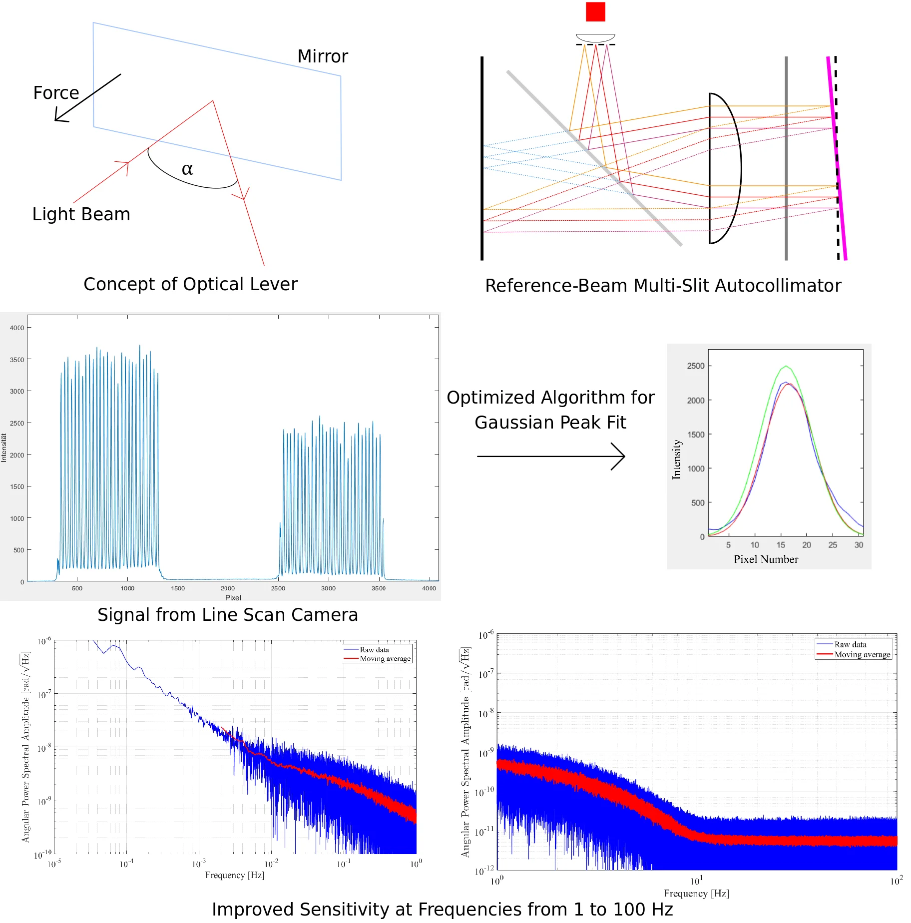
Optical levers for precision angle measurement have the advantage of exerting only a negligible force on the object being measured. Also, in autocollimating configuration, optical levers are insensitive to longitudinal movements of the target mirror. In this article, a reference-beam multi-slit autocollimator with variable number of slits, built from cost-effective off-the-shelf components, is presented. Further, an optimized algorithm for data processing is introduced, reducing computational effort for repeated Gaussian peak fitting. In the described setup, by adjusting the number of slits, the measurement range can be increased at the cost of sensitivity, and vice versa. In the tested configuration with 28 slits, the device has a measurement range of 12 mrad, and a sensitivity in the order of nrad/ starting at frequencies of 0.1 Hz, with increased sensitivity compared to other recently described autocollimators at frequencies over 1 Hz.
Highlights
- A reference-beam multi-slit autocollimator with variable number of slits is presented
- An optimized algorithm was developed for repeated Gaussian peak fitting
- Improved sensitivity was found at frequencies from 1 to 100 Hz
- The setup was built using cost-effective off-the-shelf components
1. Introduction
The first optical lever for precise and contactless angle measurement was described by Poggendorf in 1826 [1]. In 1867, Kelvin was the first to image an illuminated slit onto a scale by reflecting light at a target mirror. The combination of an optical lever with a torsion balance enabled measurements of extremely small forces and made some important experiments in the history of physics possible. Eötvös used an optical lever in autocollimating configuration with a torsion balance for measurement of gradients in terrestrial gravity and determining bounds on the violation of Einstein’s principle of equivalence of inertial and gravitational mass [2]. Later, with the introduction of photosensitive electronic detectors, the angular resolution of such devices improved significantly. In 1992, Cowsik designed an optical lever in which a slit is imaged onto a charge-coupled device (CCD). More recently, Cowsik et al. improved this setup by imaging multiple slits and thereby once more enhancing angular resolution. With this device, a resolution of 10-10 rad/ and a dynamic range exceeding a few million was achieved [2]. In 2013, Arp et al. presented a modified design of the multi-slit autocollimator, incorporating a condensing lens and a reference mirror [3]. While the condensing lens reduces optical aberrations and increases intensity, the differential measurement between reference and target mirror effectively suppresses noise sources which affect both mirrors in the same way (e.g., thermal expansion of the autocollimator body or vibration). This autocollimator design is currently being used for testing the LISA spacecraft and in a tilt sensor for the Advanced LIGO project [4].
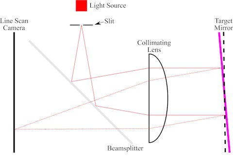
Key component of an autocollimator is the collimating lens, which collimates light from an illuminated slit into a parallel beam. For this purpose, the slit is placed in the focal plane of the collimating lens. After reflection off a target mirror the same lens is used – typically via a 50-50 beamsplitter – to image the slit onto a sensor, which is again located in the focal plane (see Fig. 1). The parallel beam reflected off the target mirror has twice the angle of interest with respect to the incident beam. Rotation of the mirror by an angle results in a displacement of the light spot on the sensor, with:
in the limit of small ,where is the focal length of the collimating lens.
Fig. 1Schematic diagram of a single-slit autocollimator
An optical lever in autocollimating configuration has the advantage of being independent of variations in the placement of the target mirror. Further, optical aberrations of the collimating lens are reduced, since the light passes the same lens on the way back to the photodetector. For these reasons, modern optical levers are typically designed as autocollimators. Different designs of this single-slit autocollimator obtain sensitivities of a few nrad/ [5, 6].
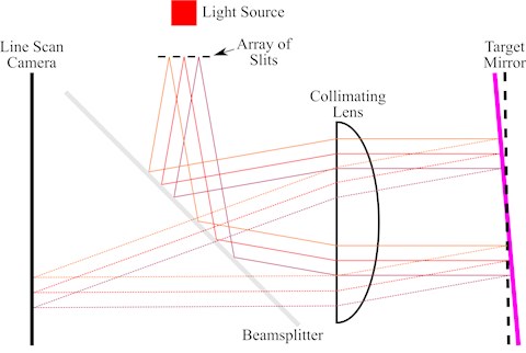
The multi-slit autocollimator developed by Cowsik et al. increases sensitivity and dynamic range compared to a standard autocollimator by imaging an array of slits via the target mirror onto a linear CCD [2] (see Fig. 2). In this configuration, multiple measurements are performed at the same time, thereby efficiently increasing the number of individual measurements, hence improving the precision of the result.
Fig. 2Schematic diagram of a multi-slit autocollimator
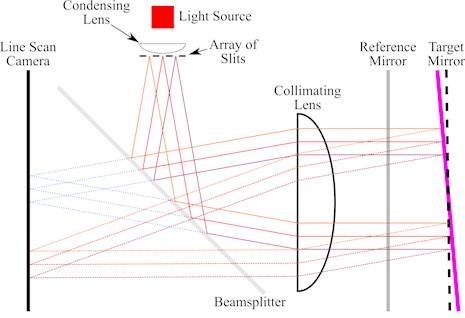
Arp et al. added two optical components to Cowsik’s design: a condensing lens and a reference mirror [3]. In this setup, the condensing lens is located between the light source and the array of slits, close to the slits (see Fig. 3). This lens reduces the divergence of the light rays, thereby increasing light intensity in the center of the collimating lens. In this way, chromatic and spherical aberrations of the collimating lens are reduced, and the slits imaged onto the detector are more uniformly illuminated. The distance between the light source and the condensing lens is adjusted so that the source is imaged onto the target mirror, establishing a symmetry between source and detector optical paths. This further reduces optical aberrations and maximizes symmetry [1, 3]. In addition to this, a partially transparent reference mirror (60T-40R) is placed in front of the target mirror. The light reflected off the reference mirror forms a second image of the slits on the CCD, acting as a reference against which the image originating from the target mirror can be compared. Obviously, this differential measurement suppresses noise that is common-mode to both the target and the reference mirrors. As reported by Arp et al., this method reduces the noise floor by an order of magnitude at frequencies below ~0.2 Hz [3].
Fig. 3Schematic diagram of a multi-slit autocollimator with condensing lens and reference mirror
In order to enhance the thermal stability of the device, Arp et al. built the autocollimator body from thick aluminum and separated the main heat sources, namely the readout electronics of the CCD camera and the light source (LED), from the body. The LED was connected to the optical path via a multimode optical fiber. Overall, in this setup the effect of temperature variation was reduced below the noise floor of 1 nrad/ for frequencies from 10 mHz to 1 Hz [3].
2. Theoretical background
Theoretical limits to the performance of a multi-slit autocollimator as well as requirements concerning spatial and intensity digitization were described in detail by Cowsik et al. [2]. In the following, only a brief summary is given and results from Cowsik et al. are analyzed with respect to the device presented here.
The image of a single slit can be assumed to have a Gaussian profile with an RMS width (standard deviation) of . This assumption also forms the basis of the peak fitting algorithm explained in Section 4. The image width is the sum of the width of the slit and the width of the diffraction pattern:
where is the central wavelength of the light source and and are the focal length and the diameter of the collimating lens, respectively. Assuming that only a single slit is used for the measurement, the resolution of the autocollimator can be estimated by calculating the uncertainty of the measurement of the center position of this peak, given by:
where is total number of photons in the image collected per second [2]. It can be seen that the resolution can be improved by increasing . However, attempting to increase the number of photons by increasing the width is frustrated by a more rapid growth in , since is proportional to (see Eq. (2)). On the other hand, the size of the slit cannot be reduced indefinitely due to diffraction at the slit that will spread the beam over a certain angle. Calculating the measurement angle according to Eq. (1) and inserting the uncertainty of yields the theoretical limit of the resolution, which depends on the diameter of the collimating lens and the intensity of the light source (see [2]):
Further improvement of the angular resolution can be obtained by imaging multiple slits onto the detector. In this case, the uncertainty of becomes:
where is the number of slits. Thus, the resolution improves by a factor . Cowsik et al. also estimated the minimum number of pixels for the image of a single slit to 6-7 pixels in order to avoid errors due to spatial digitization. Further, the bit depth of the analog-to-digital converter (ADC) should be at least 8 bit [2].
In the autocollimator setup built in this work, the image of a single slit comprises 31 pixels, and the ADC has a bit depth of 12 bit, both satisfying the criteria defined in [2]. Further, components with 50 mm diameter were chosen in order to reduce (see Eq. (2)). However, it has to be noted that Eq. (4) only holds true for an idealized detector with perfect spatial resolution. Obviously, this theoretical limit cannot be achieved by a real laboratory setup.
3. Materials and methods
The autocollimator setup described in this article is based on the work of Arp et al. [3], although the housing of our device is made out of standard components, in order to build an economically feasible device. To reduce the overall costs of the setup actually was one of the main targets of this work. Several modifications were made to the system described by Arp et al. [3]. The algorithm for data processing was improved to run in a MATLAB environment at relatively high frame rates and to provide automatic and continuous detection of reference and target patterns. Instead of a chrome photomask, a commercial grating with 40 line pairs per cm was used. An iris aperture was placed immediately in front of the grating, allowing to adjust the number of slits that are imaged onto the camera. With this method, low-cost components can be employed instead of a custom-made grating. Another advantage of this approach is, that the measurement range can be increased at the cost of sensitivity, or vice versa, in order to find the best compromise for each application. Due to the smaller pixel size of the camera (7 µm instead of 14 µm compared to Arp et al. [3] and Cowsik et al. [2]), more pixels are available for Gaussian peak fitting. Alternatively, more slits can be imaged on the same area without losing information.
Optical and mechanical components were mounted on an aluminum breadboard (Thorlabs, MB2060/M). For the long-term measurements discussed in Section 5, the breadboard was placed on a damped optical table (Thorlabs, Nexus Breadboard B90150B). As light source, a fiber-coupled LED (Thorlabs, M625F2) with 625 nm nominal wavelength and 17.5 mW output power (ex 400 µm fiber) was used. This LED was mounted to a 34 mm long heat sink, improving thermal stability. In order to prevent the LED from heating the autocollimator, it was placed about 1 m away from the optical system, connected to the optical path via a multimode fiber with 400 µm core diameter (Thorlabs, M28L01). The intensity of the LED was adjusted to allow the camera to operate at an optimum point about five to ten percent below saturation.
For the optical setup (see Fig. 4), components with 50 mm diameter (lenses and lens tubes) or 50 mm side length (beamsplitter cube) were selected, allowing the imaging of the slits onto the camera with a high cutoff frequency. This optic diameter also enables measurements at relatively large angles and distances between the autocollimator and the target and reference mirrors. In order to reduce reflections, all optic surfaces, except for the grating, have a broadband anti-reflection coating for the visible range.
Fig. 4Photograph of the optical setup: 1 – optical fiber; 2 – condensing lens; 3 – grating and iris aperture; 4 – beamsplitter cube; 5 – beam block; 6 – CMOS line scan camera; 7 – collimating lens
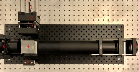
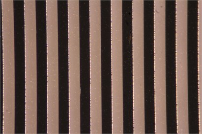
An aspheric lens with 40 mm focal length (Thorlabs, ACL5040U-A) was used as condensing lens. The grating (3B Scientific, U14103, central section with 40 line pairs per cm, see Fig. 5) was mounted immediately next to the condensing lens, with the curved surface of the lens pointing to the grating. After passing through the grating and the iris aperture, the beam was split by a 50-50 beamsplitter cube (Thorlabs, BS031) into two parts: one that was collimated by the collimating lens and one that was absorbed by the beam block (Thorlabs, LB1/M). As collimating lens, an achromatic doublet with 500 mm focal length (Thorlabs, AC508-500-A-ML) was used. The grating, as well as the camera, were placed in the focal plane of the collimating lens, about 513 mm from the back surface of the lens. This distance deviates from the nominal back focal length (496 mm), due to the optical path within the material of the beamsplitter cube (N-BK7). Using an achromatic doublet reduces the sensitivity of the autocollimator to wavelength fluctuations of the LED. Also, for the purpose of imaging a point source to infinity, this lens is practically free from spherical aberration.
Fig. 5Microscope photograph of the grating (3B Scientific, U14103)
The parallel beam originating from the collimating lens was reflected by the reference mirror (Edmund Optics, #68-393, 60T-40R) and the target mirror (Thorlabs, BB2-E02). For the measurements discussed in Section 5, the mirrors were mounted on a small breadboard located about 1 m away from the collimating lens and with 8 cm distance between reference and target mirror. The back surface of the reference mirror also had an anti-reflection coating, in order to reduce multiple reflections between the two mirrors. The reflected parallel beams were again focused by the collimating lens, and imaged – via the beamsplitter – onto the camera (and partially into the source path). The camera (Teledyne DALSA, LA-GM-04K08A) had a monochrome linear CMOS array with 4096 pixels, a pixel size of 7.04 x 7.04 µm at the nominal operating temperature (45 °C), a bit depth of up to 12 bit (used in this work), and a GigE Vision interface with a maximum line rate of 26 kHz in standard mode. Two translation stages oriented at an angle of 90 degrees allowed for fine-tuning of the focus and centering the camera with respect to the optical axis.
As mentioned before, the number of slits that are imaged onto the CMOS array can be adjusted by the iris aperture. Increasing the number of slits improves sensitivity but reduces the maximum angle that can be measured. In this work, 28 slits were imaged onto the camera for both the reference and the target mirror (56 slits overall).
4. Data processing
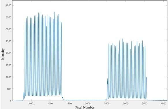
The graphical user interface (GUI) for the readout of the camera and data processing was programmed in MATLAB R2019a (The MathWorks, Inc., Natick, MA). Additionally, the Image Acquisition Toolbox was used, enabling a connection between the camera and MATLAB. The main tasks of the program are: timed acquisition of line data from the camera; detection of the peaks stemming from reference and target pattern; weighted fitting of a Gaussian curve to each peak; and calculating the angle resulting from the average difference between the corresponding peak positions of the two patterns. An example of the signal obtained from the line scan camera, i.e., the patterns reflected at the reference and the target mirror, is shown in Fig. 6.
Fig. 6Frame from the line scan camera with reference pattern (left) and target pattern (right)
The peak detection algorithm is based on finding local maxima. Pixel intensities are analyzed starting at the first pixel of the line array. As soon as the intensity exceeds a pre-defined threshold (e.g., 1100), the algorithm looks for the maximum intensity in a region, e.g., 20 pixels, following the first pixel that exceeds the threshold. The size of this region has to be chosen in a way that, based on the pixel size and the distance between the slits, the region contains exactly one local maximum. In the next step, a sub-array of pixel intensities is defined with the local maximum in the center, again containing only the signal of this slit, but not the neighboring slits. This sub-array contains the intensity data that is fitted with a Gaussian function, as will be described in the next paragraph. This method has the advantage of being unaffected by intensity fluctuations which can influence pixels to cross the threshold, since the sub-array is always centered on the local maximum.
In the next step, the parameters , , and of a Gaussian function of the form:
are fitted to the intensity data of the sub-array, where represents the height, the center, and the standard deviation of the curve. Calculating the logarithm reduces the general, nonlinear least squares problem to fitting a quadratic function:
with the coefficients:
although – for determining the angle – only is required.
Because calculating the logarithm is time-consuming and there is only a finite number of possible intensity values for each pixel , a lookup-table for the logarithm is generated at the beginning of the program, reducing the processing-time within the loop. Also, since the sub-array that is evaluated for the weighted polynomial fit has the same size for each peak, the values are the same for each run of the peak fitting loop. For example, if the sub-array has 31 pixels, the array of values is 1, 2, ..., 31, while the values are different for each run of the loop. The values for remain constant for the runtime of the program, which helps further reducing computational effort, as explained in the following paragraphs.
The least squares problem corresponding to the finding the polynomial coefficients , and can be written in the form:
where are the weights of each pixel , , and is the number of pixels in the sub-array. In matrix notation, Eq. (10) can be written as:
with the Vandermonde matrix and the coefficient vector :
One method for solving Eq. (11) is factorization of the Vandermonde matrix :
where is an orthogonal matrix (, ), and is an upper triangular matrix [7]. Thus, Eq. (11) can be written as:
leading to:
Since contains only the constant vectors and , the matrices and are constant for every iteration of the peak fitting loop. Only the vector , containing the logarithms of the intensity values , changes with each pass of the loop. This means that and can be calculated at the beginning of the program, reducing the process of fitting a Gaussian function to taking the logarithm of the intensity values via a lookup-table and two matrix multiplications. This shortens the processing time compared to calling the built-in polynomial fit function in every iteration of the loop. This method increases the rate of peak fitting by a factor of 10 to 20, enabling frame rates up to 200 Hz (400 Hz without graphical output) in the MATLAB program. Compiling the program or implementing the peak fit according to Eq. (16) in a dynamic library could further increase the performance. However, in the current application a frame rate of 10 Hz was required, which was sufficiently fulfilled by this MATLAB program.
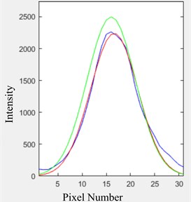
For the weights , a Gaussian function was used, approximately centered on each peak, as described by Arp et al. [3]. This function emphasizes the central part of the peak with high intensity pixels having better sensitivity and lower noise compared to peripheral pixels. Other weighting functions (triangular and trapezoidal) were tested. However, Gaussian weighting produced the best results regarding noise and stability to intensity fluctuations. An example of the weighting function, the signal of a single slit, and the Gaussian fit is shown in Fig. 7.
Fig. 7Example of weighting function (green), signal (blue) and Gaussian fit (red)
Because the number of slits imaged onto the line scan camera is variable in this setup, a simple algorithm was implemented in order to identify peaks belonging to the reference and target patterns. In the first step the distances between adjacent peaks are calculated. These distances equal the spacings between the slits of the grating for each pattern. However, the gap between the last peak of the reference signal and the first peak of the target signal is typically much larger. This fact is used by the algorithm to discriminate between the two patterns, which works reliably as long as the signals are sufficiently separated on the camera chip. The advantage of this method is, that the number of slits can be adjusted while the program is running. In case the algorithm finds a different number of peaks for the reference and the target pattern, which can occur due to the fixed threshold and the different intensities of the two patterns, the threshold is automatically adapted by the program until the algorithm finds the same number of slits for both patterns.
The resulting difference angle is then determined by calculating the mean distance between each peak of the reference pattern and the corresponding peak of the target pattern, divided by two times the focal length of the collimating lens (see Eq. (1)).
5. Results
Main aim of the measurements performed in this work was to analyze the performance of the autocollimator at different frequencies and, further, to evaluate the influence of temperature variations and air flow. For this purpose, target and reference mirrors were held in a fixed position. Measurements over several hours show that our system is prone to temperature-related drifts. However, analysis of the power spectral amplitudes shows that for frequencies over ~1 Hz our system has better sensitivity compared to the autocollimators described by other groups. A comparison of the corresponding angular power spectral amplitudes is given in Table 2.
Measurements were performed with the setup mounted on a damped optical table. The temperature during the measurements was recorded using a thermocouple temperature logger (Picotech, TC-08) in intervals of 1 minute. Thermocouple sensors were mounted close to the line scan camera, the collimating lens, and the reference mirror. Air flow and temperature of the laboratory were controlled automatically, with a reduction of air flow and cooling during night-time. An example of a measurement over 12 hours, recorded at a frame rate of 200 Hz, is shown in Fig. 8.
Fig. 8Measured difference angle (blue), moving average (red), and temperature (green) over 12 hours
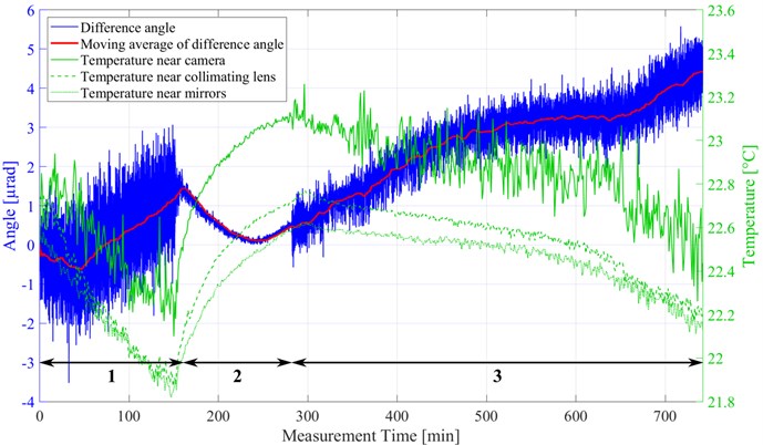
As can be seen in Fig. 8, air flow as well as temperature variations have a significant influence on the measured difference angle, increasing noise and leading to a temperature-related drift. Standard deviations of the angle calculated over time spans of 1 to 1000 seconds during normal operation of the climatization (marked with ‘1’ in Fig. 8), while the air flow was turned off overnight (marked with ‘2’), and during reduced operation (marked with ‘3’), are shown in Table 1. Standard deviations below 20 nrad are achieved for time spans up to 100 seconds while the air flow is turned off (phase 2 in Table 1). The rise in temperature during phase 2 can also be associated with a reduction of the measured angle, as can be seen in Fig. 8. Also, an underlying drift that is not directly related to room temperature was observed, which could possibly be due to wavelength fluctuations of the LED or thermal expansion of the line scan camera. Overall, the drift of the angle during this 12 hour-period was ~5 µrad, which is about a factor 25 higher than in the thermally stabilized setup built by Arp et al. [3].
Table 1Standard deviation of difference angle
Time span [s] | Standard deviation [nrad] | ||
Phase 1 | Phase 2 | Phase 3 | |
1 | 209 | 8 | 21 |
10 | 345 | 11 | 82 |
100 | 448 | 18 | 148 |
1000 | 452 | 57 | 203 |
The power spectral amplitude, corresponding to the angular resolution of the system at different frequencies, is calculated via the complex magnitude of the fast Fourier transform (FFT) divided by half the number of data points. Power spectral amplitudes for the measurement shown in Fig. 8 are given in Fig. 9 (lower frequencies up to 1 Hz) and Fig. 10 (higher frequencies up to 100 Hz). A comparison of these amplitudes to the results obtained by Arp et al. [3] and Cowsik et al. [2] is shown in Table 2. Data for [2, 3] in Table 2 were estimated from the figures in the respective publications.
Fig. 9Angular power spectral amplitude at lower frequencies: raw data (blue) and moving average (red)
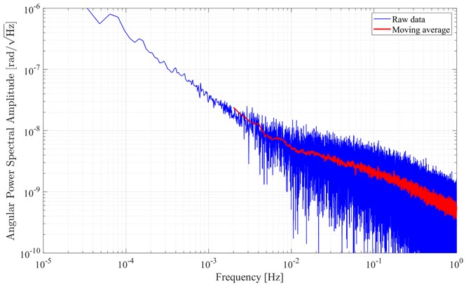
In contrast to the described system, which was made out of standard components and not fully enclosed within a housing, the devices built by Arp et al. [3] and Cowsik et al. [2] used dedicated aluminum housings, giving them long thermal time constants. Moreover, air flow increased the noise level in the measurement, as is shown in Table 1. Thus, for low frequencies up to 1 Hz, angular power spectral amplitudes of the measurements presented here are approximately a factor 5 to 10 higher than the amplitudes of the other systems, as can be seen in Table 2. However, at frequencies over 10 Hz the resolution of our setup is about 1 to 2 orders of magnitude better than the resolution of the other systems, reaching 6 prad/ for frequencies over 15 Hz. This can probably be attributed to the different technologies of the line scan cameras (readout electronics, pixel size of 7 µm vs. 14 µm, bit depth, or CMOS vs. CCD) or – in comparison to Cowsik et al. [2] – a different algorithm (weighted Gaussian peak fit vs. centroid algorithm). Further studies are required to investigate this phenomenon. Table 3 shows an overview of the pitch, the pixel sizes and the number of evaluated pixels for the different autocollimators discussed here. It can be seen that, although our system images less slits than the other devices, due to the smaller pixel size more pixels are evaluated. This is probably one of the reasons for the good performance of this autocollimator setup at higher frequencies.
Fig. 10Angular power spectral amplitude at higher frequencies: raw data (blue) and moving average (red)
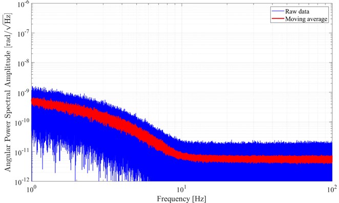
Table 2Comparison of angular power spectral amplitudes
Frequency [Hz] | Angular power spectral amplitude [rad/ | ||
ACMIT setup | Arp et al. [3] | Cowsik et al. [2] | |
10-4 | 4×10⁻⁷ | 1×10⁻⁷ | 3×10⁻⁸ |
10-3 | 4×10⁻⁸ | 6×10⁻⁹ | 2×10⁻⁹ |
10-2 | 5×10⁻⁹ | 1×10⁻⁹ | 2×10⁻¹⁰ |
10-1 | 2×10⁻⁹ | 1×10⁻⁹ | 2×10⁻¹⁰ |
100 | 5×10⁻¹⁰ | 1×10⁻⁹ | 2×10⁻¹⁰ |
101 | 7×10-12 | 1×10⁻⁹ | 2×10⁻¹⁰ |
102 | 6×10-12 | 1×10⁻⁹ | – |
Table 3Comparison of gratings, pixel sizes and number of evaluated pixels
System | Pitch [µm] | Pixel size [µm] | Pixels per slit | Number of slits | Evaluated pixels |
ACMIT | 250 | 7.04×7.04 | 31 | 2×28 | 2×868 |
Arp et al. [3] | 290 | 14×14 | 19 | 2×38 | 2×722 |
Cowsik et al. [2] | 182 | 14×14 | 13 | 110 | 1430 |
6. Conclusions
In this work we present a reference-beam multi-slit autocollimator built from standard components, which is able to achieve resolutions in the sub-nanoradian range for frequencies over 1 Hz. In this setup, the number of slits imaged onto the line scan camera can be adjusted by an iris aperture. A larger aperture increases sensitivity but reduces the measurement range, and vice versa. A measurement range of 12 mrad is obtained with 28 slits imaged onto the camera for both the reference mirror and the target mirror. The grating, which is a low-cost off-the-shelf component, has sufficient quality for this application. The optimized algorithm, which reduces processing time of a repeated Gaussian peak fit for constant weights and -values, allows for frame rates up to 400 Hz in MATLAB.
Long-term measurements show the limitations of the system, particularly the sensitivity of the device to temperature changes in an ambient environment. Temperature-related drifts are, although acceptable for some applications, higher than the drifts observed by other groups working with thermally stabilized setups. The maximum sensitivity of our autocollimator is achieved at frequencies over 15 Hz, compared to approximately 10 mHz in the thermally stable system designed by Arp et al. [3]. On the other hand, the resolution of our autocollimator at frequencies over 10 Hz is up to 2 orders of magnitude better than the resolutions of the other systems discussed here, with 6 prad/ for frequencies over 15 Hz, indicating very good short-term performance of our device. We are confident that a major part of the improvement found in this work is due to the line scan camera used here.
References
-
Jones R. V. Some developments and applications of the optical lever. Journal of Scientific Instruments, Vol. 38, 1961, p. 37-45.
-
Cowsik R., Srinivasan R., Kasturirengan S., Senthil Kumar A., Wagoner K. Design and performance of a sub-nanoradian resolution autocollimating optical lever. Review of Scientific Instruments, Vol. 78, 2007, p. 035105.
-
Arp T. B., Hagedorn C. A., Schlamminger S., Gundlach J. H. A reference-beam autocollimator with nanoradian sensitivity from mHz to kHz and dynamic range of 107. Review of Scientific Instruments, Vol. 84, 2013, p. 095007.
-
Venkateswara K., Hagedorn C. A., Turner M. D., Arp T., Gundlach J. H. A high-precision mechanical absolute-rotation sensor. Review of Scientific Instruments, Vol. 85, 2014, p. 015005.
-
Smith G. L., Hoyle C. D., Gundlach J. H., Adelberger E. G., Heckel B. R., Swanson H. E. Short-range tests of the equivalence principle. Physical Review D, Vol. 61, 1999, p. 022001.
-
Pollack S. E., Schlamminger S., Gundlach J. H. Temporal extent of surface potentials between closely spaced metals. Physical Review Letters, Vol. 101, 2008, p. 071101.
-
Moler C. Numerical Computing with MATLAB. The MathWorks, Natick, MA, 2004.
About this article

The authors would like to thank Christian Krutzler from ACMIT Gmbh and Martin Gröschl from the Vienna University of Technology for supporting this research project. Valuable discussions with Kirsten Lux, Wolfgang Brezna, Wolfgang Göb, and Johanna Spielauer are acknowledged.
This work has been supported by ACMIT – Austrian Center for Medical Innovation and Technology, which is funded within the scope of the COMET – Competence Centers for Excellent Technologies program and funded by the federal government of Austria and the governments of Lower Austria and Tyrol. The competence center program COMET is managed by the Austrian Funding Agency FFG.
Financial support from the government of Lower Austria (grant number K3-F-807/001-2018) is gratefully acknowledged.
