Abstract
In order to ensure the safety of bridge structure operation, the working mechanism and damage mechanism of spherical steel bearings commonly used in urban rail transit bridges and large highway bridges are studied. This study combines correlation and sensitivity analysis methods, and proposes that the correlation between output parameters and input parameters and the order of sensitivity are used as the basis for selecting spherical steel bearings. The sudden change of the sensitivity of each operating point is used as the basis for index division, and the discriminating system of spherical steel bearings is established accordingly. Combined with SVM, it is trained into a ball-type steel bearing safety level discrimination model. Through the test data test, the results show that the test of the discriminant model is effective.
Highlights
- A method for establishing an evaluation system based on SVM is proposed.
- Use input parameters and output parameters as the data to establish SVM.
- Realize the purpose of crossing the intermediate parameters from input parameters to output parameters.
- This method not only improves the efficiency of rating, but also starts from the calculation and analysis of structural performance to rate structural members.
1. Introduction
Bridge bearing is an essential component in bridge structures. Bridge bearings are used in many bridge designs and constructions. The central role of bridge bearings in the bridge structure is to bear the dead weight from the superstructure and other live loads generated vertically, longitudinally and laterally by the bridge, and transfer these loads to the substructure. Bridge bearing bears part of the deformations such as displacements and rotation angles caused by these loads. At present, there is no precise quantitative index and evaluation system for the working performance of bridge bearing. In urban rail transit, railway bridges, and long-span highway bridges, because of the higher demand for the angle, displacement, and life of the selected bridge support, spherical steel supports often become the primary choice because of their structural characteristics. However, there are few studies on the working mechanism, damage mechanism, and damage mechanism of spherical bearings.
Wang Hui [1] proposed a method for dynamic identification of bridge bearings based on Fourier transform confidence criterion and model modification theory based on the theory of modal parameter damage identification. Qiao Zhen [2] proposed a method to detect the damage of bridge supports using the frequency change rate based on the theory of bridge vibration. Yin Qiang [3] studied the Kalman filter and sequential non-linear least-squares method, and proposed an adaptive tracking technology based on the optimization method to identify the system parameters of the rubber-isolated bearing and its structure online, so that Determine the occurrence of structural damage. Doebling W. et al. [4] also proposed a method for structural damage identification based on the structural vibration theory. Guo Jian et al. [5] studied the application of wavelet analysis theory to damage identification of bridge supports, combined with the correlation function of structural dynamic response, constructed a new damage index, combined with the continuous beam bridge in Zhoushan Cross-sea Bridge, Zhejiang Vibration characteristics, model test research of bearing damage is designed and carried out. The sensitivity of each damage index to identify bearing damage is analyzed.
According to the research status of bridge bearings and their damage indicators, although there are currently many evaluation methods or evaluation indicators, none of them is a systematic proposal of a bridge bearing evaluation system from the perspective of the bearing performance of the bridge bearings. Based on the correlation and sensitivity analysis theories and methods, this paper proposes to use the correlation between the output parameters and the input parameters and the order of the sensitivity as the basis for selecting the discriminating indicators for the spherical bearings. A large number of working condition simulations seek the critical points of the damage index, and based on this, a spherical bearing identification system is established. This paper uses a large number of operating point calculations to directly determine the practical performance level of the spherical bearing from the magnitude of the stress according to the established damage evaluation system. It corresponds one-to-one with the vertical and shear loads of the spherical bearing. This paper combines SVM to form a model for determining the safety level of spherical bearings.
2. Vertical load test and data analysis of spherical bearing
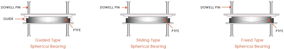
This test uses a YJW-20000 pressure testing machine with a maximum load of 20MN, and the test product is JQZ I 5.0 SX. The photos of the experimental site and facilities are shown in Fig. 1. This type of bearing is a sliding type spherical bearing with a vertical design load of 5MN, a horizontal design load of 500 kN, and a design rotation angle of 0.02 rad. The overall assembly diagram is shown in Fig. 2. In order to study the vertical behavior of the component and the deformation of the basin under the vertical load, a vertical bearing capacity test was performed on the product according to the test regulations [6]. In addition, for ease of understanding, a schematic diagram of the guided type spherical bearing structure is shown in Fig. 3. The difference between guided-type spherical bearing, sliding-type bearing, and fixed-type bearing is shown in Fig. 4.
Fig. 1The experimental site and facilities
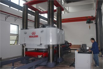
a) Test facilities
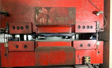
b) Test site
Fig. 2JQZ I 5.0 SX assembly diagram (unit: mm)
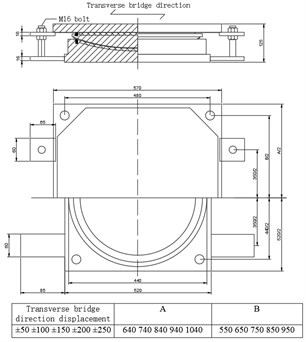
Fig. 3Spherical bearing structure
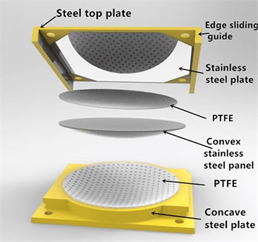
Table 1Three sets of experimental data
Bearing sample | Specimen number | Test Date | GB/T17955-2009 | ||||||||||
Bearing model | JQZ I 5.0SX | ||||||||||||
Bearing height (mm) | 125.00 | Bearing outer diameter (mm) | 515.00 | ||||||||||
Testing facilities | YJW-20000 | ||||||||||||
Testing date | Temperature | 25 °C | |||||||||||
Measurement times | Displacement sensor number | Vertical compression deformation (mm) nuder step loading (kN) | |||||||||||
25 | 750 | 1500 | 2250 | 3000 | 3750 | 4500 | 5000 | 6000 | 6750 | 7500 | 25 | ||
1 | N1 | 0.360 | 0.482 | 0.592 | 0.695 | 0.797 | 0.897 | 0.986 | 1.043 | 1.155 | 1.24 | 1.331 | 0.392 |
N2 | 0.601 | 0.745 | 0.890 | 1.03 | 1.177 | 1.313 | 1.448 | 1.545 | 1.739 | 1.89 | 2.055 | 0.731 | |
N3 | 0.114 | 0.835 | 0.935 | 0.984 | 1.008 | 1.026 | 1.037 | 1.038 | 1.043 | 1.048 | 1.053 | 0.093 | |
N4 | 0.280 | 1.016 | 1.161 | 1.26 | 1.338 | 1.402 | 1.468 | 1.511 | 1.608 | 1.686 | 1.769 | 0.361 | |
Average reading | 0.339 | 0.770 | 0.895 | 0.992 | 1.080 | 1.160 | 1.235 | 1.284 | 1.386 | 1.466 | 1.552 | 0.394 | |
Deformation (mm) | 0.431 | 0.556 | 0.653 | 0.741 | 0.821 | 0.896 | 0.945 | 1.047 | 1.127 | 1.213 | 0.055 | ||
Deformation percentage | 0.344 | 0.444 | 0.523 | 0.593 | 0.656 | 0.717 | 0.756 | 0.838 | 0.902 | 0.970 | 0.044 | ||
2 | N1 | 0.392 | 0.503 | 0.612 | 0.714 | 0.817 | 0.916 | 1.005 | 1.063 | 1.168 | 1.242 | 1.321 | 0.380 |
N2 | 0.731 | 0.848 | 0.998 | 1.140 | 1.285 | 1.420 | 1.555 | 1.648 | 1.830 | 1.962 | 2.108 | 0.807 | |
N3 | 0.093 | 0.826 | 0.919 | 0.967 | 0.990 | 1.012 | 1.024 | 1.027 | 1.027 | 1.030 | 1.031 | 0.069 | |
N4 | 0.361 | 1.090 | 1.235 | 1.333 | 1.411 | 1.477 | 1.542 | 1.587 | 1.671 | 1.739 | 1.811 | 0.425 | |
Average reading | 0.394 | 0.817 | 0.941 | 1.039 | 1.126 | 1.206 | 1.282 | 1.331 | 1.424 | 1.493 | 1.568 | 0.420 | |
Deformation (mm) | 0.423 | 0.547 | 0.645 | 0.732 | 0.812 | 0.888 | 0.937 | 1.030 | 1.099 | 1.174 | 0.026 | ||
Deformation percentage | 0.338 | 0.438 | 0.516 | 0.585 | 0.650 | 0.710 | 0.750 | 0.824 | 0.879 | 0.939 | 0.021 | ||
3 | N1 | 0.380 | 0.502 | 0.611 | 0.712 | 0.815 | 0.914 | 1.002 | 1.059 | 1.165 | 1.238 | 1.316 | 0.367 |
N2 | 0.807 | 0.905 | 1.056 | 1.199 | 1.344 | 1.478 | 1.610 | 1.703 | 1.880 | 2.010 | 2.147 | 0.863 | |
N3 | 0.069 | 0.812 | 0.903 | 0.949 | 0.972 | 0.993 | 1.005 | 1.007 | 1.010 | 1.773 | 1.015 | 0.051 | |
N4 | 0.425 | 1.136 | 1.280 | 1.378 | 1.453 | 1.519 | 1.583 | 1.627 | 1.710 | 1.508 | 1.841 | 0.473 | |
Average reading | 0.420 | 0.839 | 0.963 | 1.060 | 1.146 | 1.226 | 1.300 | 1.349 | 1.441 | 1.632 | 1.580 | 0.439 | |
Deformation(mm) | 0.419 | 0.543 | 0.640 | 0.726 | 0.806 | 0.880 | 0.929 | 1.021 | 1.212 | 1.160 | 0.019 | ||
Deformation percentage | 0.335 | 0.434 | 0.512 | 0.581 | 0.645 | 0.704 | 0.743 | 0.817 | 0.970 | 0.928 | 0.015 | ||
Residual deformation percentage (%) | 1st | 0.044 | 2nd | 0.0208 | 3rd | 0.0152 | |||||||
Measurement times | Displacement sensor number | Deformation (mm) of the upper mouth of the lower basin ring in step loading (kN) | |||||||||||
25 | 750 | 1500 | 2250 | 3000 | 3750 | 4500 | 5000 | 6000 | 6750 | 7500 | 50 | ||
1 | L1 | 0.035 | 0.070 | 0.079 | 0.085 | 0.089 | 0.092 | 0.094 | 0.095 | 0.100 | 0.104 | 0.109 | 0.048 |
L2 | -0.016 | -0.003 | 0.004 | 0.009 | 0.015 | 0.019 | 0.023 | 0.025 | 0.032 | 0.037 | 0.043 | -0.013 | |
L3 | 0.024 | 0.025 | 0.028 | 0.030 | 0.033 | 0.034 | 0.036 | 0.037 | 0.040 | 0.044 | 0.048 | 0.026 | |
L4 | -0.020 | -0.005 | 0.003 | 0.009 | 0.014 | 0.018 | 0.021 | 0.023 | 0.027 | 0.030 | 0.035 | -0.023 | |
Average reading | 0.006 | 0.022 | 0.029 | 0.033 | 0.038 | 0.041 | 0.044 | 0.045 | 0.050 | 0.054 | 0.059 | 0.010 | |
Deformation(mm) | 0.016 | 0.023 | 0.027 | 0.032 | 0.035 | 0.038 | 0.039 | 0.044 | 0.048 | 0.053 | 0.004 | ||
Deformation percentage | 0.031 | 0.044 | 0.053 | 0.062 | 0.067 | 0.073 | 0.076 | 0.085 | 0.093 | 0.102 | 0.007 | ||
2 | L1 | 0.048 | 0.074 | 0.081 | 0.086 | 0.090 | 0.093 | 0.096 | 0.098 | 0.102 | 0.105 | 0.108 | 0.048 |
L2 | -0.013 | -0.001 | 0.007 | 0.014 | 0.019 | 0.023 | 0.027 | 0.029 | 0.036 | 0.039 | 0.043 | -0.013 | |
L3 | 0.026 | 0.028 | 0.031 | 0.034 | 0.035 | 0.038 | 0.040 | 0.041 | 0.044 | 0.044 | 0.047 | 0.027 | |
L4 | -0.023 | 0.056 | 0.002 | 0.009 | 0.015 | 0.019 | 0.024 | 0.026 | 0.033 | 0.033 | 0.036 | -0.024 | |
Average reading | 0.010 | 0.039 | 0.030 | 0.036 | 0.040 | 0.043 | 0.047 | 0.049 | 0.054 | 0.055 | 0.059 | 0.010 | |
Deformation (mm) | 0.029 | 0.020 | 0.026 | 0.030 | 0.033 | 0.037 | 0.039 | 0.044 | 0.045 | 0.049 | -0.001 | ||
Deformation percentage | 0.057 | 0.039 | 0.050 | 0.058 | 0.065 | 0.071 | 0.075 | 0.085 | 0.088 | 0.094 | -0.001 | ||
3 | L1 | 0.048 | 0.073 | 0.079 | 0.084 | 0.089 | 0.092 | 0.095 | 0.097 | 0.101 | 0.104 | 0.107 | 0.049 |
L2 | -0.013 | -0.001 | 0.007 | 0.014 | 0.019 | 0.023 | 0.027 | 0.030 | 0.037 | 0.040 | 0.044 | -0.013 | |
L3 | 0.027 | 0.028 | 0.030 | 0.034 | 0.035 | 0.038 | 0.040 | 0.041 | 0.044 | 0.044 | 0.047 | 0.027 | |
L4 | -0.024 | -0.009 | 0.001 | 0.009 | 0.015 | 0.019 | 0.024 | 0.026 | 0.031 | 0.033 | 0.036 | -0.024 | |
Average reading | 0.010 | 0.023 | 0.029 | 0.035 | 0.040 | 0.043 | 0.047 | 0.049 | 0.053 | 0.055 | 0.059 | 0.010 | |
Deformation (mm) | 0.013 | 0.019 | 0.025 | 0.030 | 0.033 | 0.037 | 0.039 | 0.043 | 0.045 | 0.049 | 0.000 | ||
Deformation percentage | 0.025 | 0.037 | 0.049 | 0.057 | 0.064 | 0.071 | 0.075 | 0.084 | 0.088 | 0.094 | 0.000 | ||
Remarker: | |||||||||||||
Inspector: | Checker: | ||||||||||||
Experiments were carried out according to the above design. Three sets of experimental data were obtained as Table 1, and two sets of unreasonable data were eliminated. The vertical deformation of the spherical bearing under the vertical load and the radial deformation of the concave steel plate, as shown in Fig. 5.
Fig. 4Schematic diagram of the three types spherical bearing structure
The load-deformation curve of the spherical bearing shown in Fig. 5 under the vertical load changes linearly. The reason for this phenomenon is that the spherical bearing is mainly made of steel, and the deformation shows the mechanical characteristics of the steel used. This feature also provides convenience for further analysis of the mechanical properties of spherical bearings.
Fig. 5Spherical bearing vertical compression and radial deformation of concave of steel plate
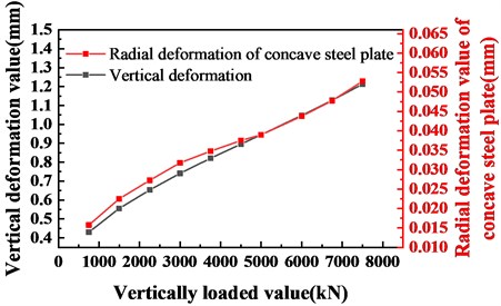
Fig. 6Ratio of vertical compression deformation value to radial deformation value of concave steel plate
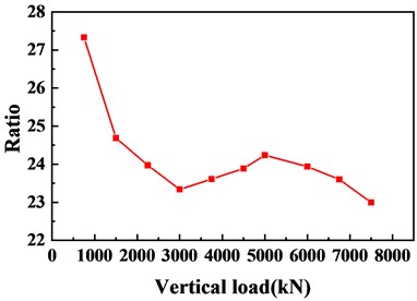
Fig. 6 shows the ratio of the vertical deformation of the spherical steel bearing to the radial deformation of the concave steel plate under vertical load. From Hooke’s law, this ratio can be approximated to represent the ratio of the vertical compression stiffness to the lateral deformation stiffness. It can be seen from the figure that 0.6 times the design load point and 1.0 times the design load point are local extreme points, and 0 times the design load point and 1.5 times the design load point are global extreme points. The reason for considering the occurrence of extreme points is due to the change in the internal structure of the bearing at the corresponding load point, so the design load points of 0 times, 0.6 times, 1.0 times, and 1.5 times are used as the basis for dividing the index threshold.
3. Finite model and test data of spherical steel rubber bearing
Establish a finite element model as shown in Fig. 7 and Fig. 8. The finite element analysis software uses ANSYS Workbench 19.0. The bearing, bolt assembly and concrete foundation are solid units Solid187, and the contact units are Contac174 and Targe170. The coefficient of friction between steel and concrete is 0.4, the coefficient of friction between steel and steel is 0.15, and the coefficient of friction between steel and polytetrafluoroethylene is 0.05. The FEM meshing diagram as shown in Fig. 7.
Fig. 7FEM meshing
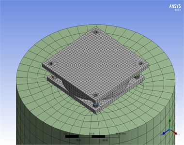
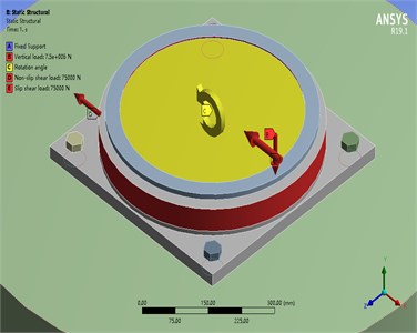
Fig. 8FEM loads and boundary conditions
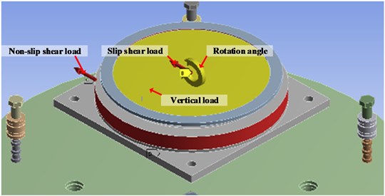
In order to simulate the working condition of the actual spherical bearing, in addition to modeling the spherical bearing, a circular concrete foundation with a diameter of 1.2 m and a height of 1.0 m was also used to simulate the pier. Among them, the concrete foundation size is determined according to the research conclusions of Zhuang Junsheng [7] and others. According to the load transmission mechanism of the spherical bearing, it can be known that the non-sliding shear load acts on the upper bearing plate and is transmitted from the upper bearing plate to the concave steel plate. The concave steel plate is transmitted to the bridge pier through bolts and friction after bearing, and the vertical load acts The upper bearing plate is transmitted to and from the ball cap liner, and then to the pier through the concave steel plate. Deformation (rotation angle and displacement) loads are also transmitted through the two methods described above, as shown in Fig. 9.
Fig. 9Schematic diagram of finite element model vertical load, shear load and rotation angle application
Through simplification, vertical load, sliding shear load and deformation (rotation, displacement) are respectively applied to the ball cap liner, and non-sliding shear load is applied to the concave steel plate, as shown in Fig. 7.
The load and boundary conditions are shown in the Fig. 8. Among them, fixed constraints are imposed on the bottom of the concrete. The rest of the load and direction are shown in the figure and described above, and the value range is shown in Table 2.
Table 2Input parameter value range
Input parameters | Vertical load | Horizontal shear load | Rotation angle |
Range | 0-5000 kN | 0-500 kN | 0-0.02 rad |
4. Evaluation and classification of spherical bearings based on correlation, sensitivity analysis and SVM
By analyzing the correlation and sensitivity of the input and output parameters of the spherical bearing under various working conditions, find the component with the lowest safety factor (such as stress close to the yield value), and affect the sensitivity of this component's safety performance Factors are sorted, and certain factors with larger sensitivity values are selected as indicators of damage. Then the changing relationship between the input factor and the selected component characterization safety value is sought, and the damage index is divided. Among them, the input parameters are vertical compressive load, horizontal shear load (including sliding shear load and fixed shear load), and the angle of the spherical bearing. The output parameters are the maximum equivalent stress of the concave steel plate, the maximum equivalent stress of the convex stainless steel plate, and the maximum shear stress of the bolt. The input parameters are determined to be 0 to 1.5 times the design load according to the relevant specifications [1] and the design value of the spherical bearing, and the vertical load is 0.1 times the shear load acting on the concave steel plate. The spherical friction coefficient of the first and second sliding surfaces is 0.03-0.05, and the spherical friction coefficient is 1.27-1.60 times the planar friction coefficient. It can be known that the shear load of the ball bearing base is far greater than the horizontal load required to overcome friction. Therefore, the calculation based on the shear load of the concave steel plate meets and covers the mechanical performance of the fixed and sliding bearing.
Select the data collection of 100 operating condition points within the specified input parameter range of the spherical bearing to perform correlation and sensitivity analysis, as shown in Figs. 10 and 11.
Fig. 10Linear correlation matrix
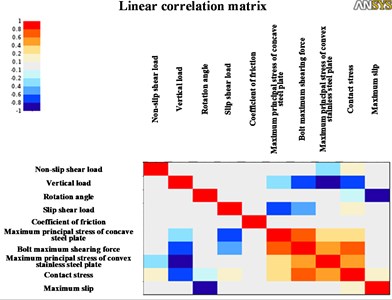
Fig. 11Quadratic correlation matrix
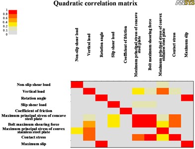
According to Figs. 10 and 11, it can be seen that the vertical load in the input parameters and the maximum principal stress value of the concave steel plate, the maximum shear stress value of the bolt and the maximum equivalent stress value of the convex stainless steel plate in the output parameter are strongly correlated. The horizontal fixed shear load in the input parameters is strongly related to the maximum equivalent stress of the concave steel plate and the maximum shear load of the bolts in the output parameters. There is a strong correlation between the sliding shear load in the input parameter and the maximum principal stress of the spherical cap liner in the output parameter. The correlation between the turning angle in the input parameter and the maximum equivalent stress value of the concave steel plate, the maximum shear stress value of the bolt, and the maximum equivalent stress value of the convex stainless steel plate in the output parameter is weak. The maximum sliding distance of the second sliding surface in the output parameter is mainly related to the rotation angle, the friction coefficient in the input parameter in the input parameter, and the sliding horizontal shear load.
Fig. 12Sensitivity relationship of input parameters to output
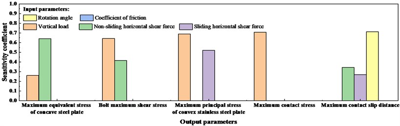
Further, as shown in Fig. 12, it can be known from the sensitivity analysis that the maximum equivalent stress of the concave steel plate, the maximum shear stress of the bolt, and the maximum equivalent stress of the convex stainless steel plate are integrated. The obvious effects on the maximum equivalent stress of the concave stainless steel plate and the maximum shear stress of bolts are vertical load and non-slip horizontal shear load. The obvious effects on the maximum equivalent stress of convex stainless steel plate are vertical load and sliding horizontal shear load. The more obvious influence on the change of contact stress is the vertical load. The most obvious impacts on the most substantial sliding amount are non-slip shearing load, sliding horizontal shearing load, and rotation angle.
Fig. 13Stress diagram of concave steel plate, bolt and convex stainless steel plate under vertical load
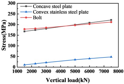
Fig. 14Stress diagram of concave steel plate, bolt and convex stainless steel plate under shear load
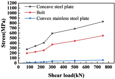
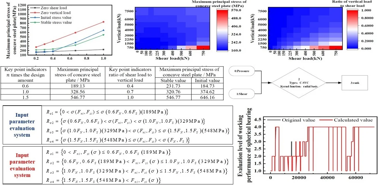
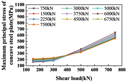
In order to further determine the magnitude of the impact of input parameters on the different support members to facilitate the division of the damage scale, the stress curves of different members of the same support under vertical and shear loads are plotted separately, as shown in Fig. 13, Fig. 14 shows. It can be seen from Figs. 13 and 14 that the maximum principal stress value of the concave steel plate is not significantly different from the maximum shear stress value of the bolt under the vertical load, and the maximum principal stress of the concave steel plate is high under the action of the shear load. The maximum shear stress of the bolt and the performance of the 8.8 type shear bolt material is better than the performance of the concave steel plate in the bearing type. Therefore, in this type of support, the maximum stress value of the concave steel plate is used as the judgment index. Includes stress values for bolts, convex stainless steel plates, and ensures the overall safety of the support. From the sensitivity analysis above, it can be seen that the input parameters of vertical load and shear load have a significant effect on the maximum principal stress of the concave plate of the spherical bearing, so the shear load and vertical load are input into the finite element model in multiple proportions. Calculate and draw the stress curve, as shown in Fig. 15.
Fig. 15Stress diagram of concave steel plate with different ratio of shear load to vertical load
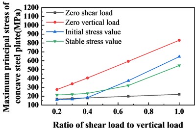
It can be seen from Fig. 15 that when the vertical load and the shear load are input in a ratio, both the initial stress value and the stable stress value are under the maximum principal stress generated by the shear load alone. And basically above the maximum principal stress of the concave steel plate under a single vertical load. It can be seen that the stress values generated under various working conditions are within this range, and the most unfavorable working conditions are generated under the maximum shear load alone. In addition, it can be seen that when calculated according to the ratio of different shear loads to vertical loads, the stress value and ratio of the generated concave steel plate are monotonically increasing. That is, the more obvious the effect of the shear load, the greater the stress of the concave steel plate. Further, in order to verify the conclusion, the maximum principal stress of the concave steel plate and the ratio of the shear load to the vertical load at different shear load to vertical load ratios were calculated. The parallel heat map is shown in Fig. 16 and Fig. 17.
Fig. 16Stress heat map of concave steel plate when different ratios of vertical load and shear load are input
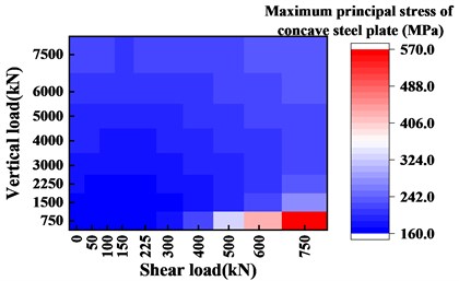
Fig. 17Heat maps with different ratios of vertical load to shear load
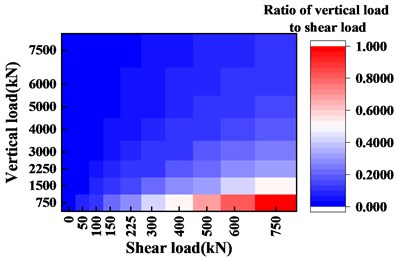
It can be seen from Fig. 16 and Fig. 17 that the results are consistent with the above conclusions. Besides, draw the stress diagram of the concave steel plate under the effect of different shear loads, as shown in Figs. 18 and 19. It can be seen that at a shear load of 300 kN and a shear load of 750 kN, the stress of the concave steel plate increases significantly. Besides, this set of data is plotted with the shear load as the horizontal axis, as shown in Figs. 13 and 14. Regarding Fig. 15, it can be concluded that the influence of the shear load and the vertical load on the concave steel plate is changed when the shear load and the vertical load are between 0.6 times the design value and 1.0 times the design value. The specific manifestation is that before the shear load of 0.6 times and the vertical load, the contribution of the vertical load to the maximum principal stress of the concave steel plate is higher than the shear load. After 1.0 times the design load, the shear load becomes the dominant factor for the maximum principal stress of the concave steel plate.
Fig. 18Stress diagram of the basin under vertical load and shear load (horizontal axis is vertical load)
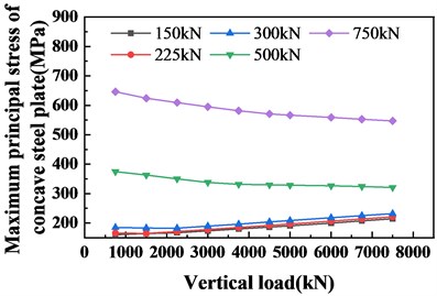
Fig. 19Stress diagram of the basin under vertical and shear loading (horizontal axis is the shear load)
Further, it can be found that the change, as mentioned above, occurs in the ratio of corresponding shear load to vertical load between 0.4 and 0.7. According to the above conclusions, in addition to the starting and ending points, two key mutation points can be determined by two methods. The first is the load design value of 0.6 times and the load design value of 1.0 times. Secondly, the stability and initial values of the concave steel plates corresponding to the shear load and vertical load ratios of 0.4 and 0.7 are used as the critical points of the damage index level of the branch seat. The list is as follows. It can be seen from Table 3 that the sum of the stress values of the concave steel plates generated by the design amount of 0.6, 1.0 times, and 1.5 times is smaller than the sum of the stress values of the concave steel plates generated by the respective shear load and vertical load ratios of 0.4, 0.7, and 1.0. In order to ensure the high security of the bearing rating, the smaller sum is selected.
Table 3Comparison table of the maximum principal stress of the concave steel plate at the key points
Key point indicators times the design amount | Maximum principal stress of concave steel plate / MPa | Key point indicators ratio of shear load to vertical load | Maximum principal stress of concave steel plate / MPa | |
Stable value | Initial value | |||
0.6 | 189.13 | 0.4 | 231.73 | 184.73 |
1.0 | 328.56 | 0.7 | 320.76 | 374.62 |
1.5 | 546.77 | 1.0 | 546.77 | 646.16 |
According to the above, the safety level of the spherical bearing is divided into four levels according to the change of vertical load and shear load, as shown in Eq. (1):
A set of vertical load and shear load data is input into the finite element model to obtain a corresponding set of concave steel plate stress values . Then, the obtained stress value of the concave steel plate is compared with the division scale of the rating index described above to obtain the rating of the support. Combining the above formula and table, specific to this column is to input array into the finite element model to obtain array . The rating scale of the rating indicators in this column is:
Through the collation of a large number of calculation data, the corresponding relationship between the vertical input load, the shear load, and the calculation grade of the spherical bearing are determined. Based on SVM training, a final discriminant model for spherical bearings is obtained:
For this example, the specific SVM training results are as follows. For classification problems under non-linear conditions, the basic idea of support vector machines is to achieve mapping from low to high dimensions through kernel functions. Then use the support vector machine to perform linear classification in the high-dimensional feature space, which is realized by the kernel function. The kernel functions commonly used now include linear kernel functions, Gaussian radial basis kernel functions, polynomial kernel functions, and exponential radial kernel functions. The support vector opportunities generated by different kernel functions are used to obtain different classification and prediction results.
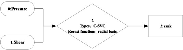
For the classification of the working state of the spherical bearing, the SVM setting type is C-SVC, the kernel function type is Gaussian radial basis, the kernel function is, the degree of the kernel function is 3, and the kernel function is The gamma function is 1/3, the coef0 in the kernel function is 0, the loss function cost is 1, and the allowable termination criterion epsilon is set to 0.001. Another 75,000 training data, because the amount of data is too large to add. The network structure is shown in Fig. 20.
Fig. 20Training structure of spherical bearings
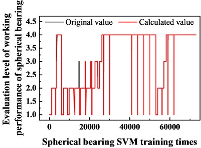
The deviation curve is shown in Fig. 21. It can be seen from the figure that the original value of the support level is different from the calculated value of the spherical support level. However, the results show that the deviation is controlled within 5 %, and the accuracy rate is above 95 %, which meets the requirements of engineering use.
Fig. 21Training deviation table for spherical bearings
5. Test verification
Further, in order to verify the correctness, seven sets of data were randomly selected and calculated as shown in Table 4, and the correct rate of judgment was all 100 %. According to the presumption of the unique points and the rating method, level 1 indicates that the spherical bearing works well. A rating of 2 indicates that the ball bearing is working correctly. Level 3 indicates that the spherical bearing is in a critical stress state. Level 4 indicates that the spherical bearing is under abnormal load and needs to be checked to determine whether it is damaged for repair and replacement.
Table 4Calculation table for program test conditions
Vertical load / kN | Shear load / kN | Judgment level | Correct rate |
2451 | 500 | 2 | 1 |
2451 | 236 | 1 | 1 |
4580 | 260 | 2 | 1 |
4500 | 150 | 1 | 1 |
5369 | 450 | 2 | 1 |
4569 | 560 | 3 | 1 |
7850 | 780 | 4 | 1 |
6. Conclusions
By studying and analyzing the working mechanism and damage mechanism of spherical bearings, the following conclusions can be obtained: (1) The core and weak parts of the spherical support are concave steel plates. The relationship between the stress value of the concave steel plate and the vertical load and the shear load is that the larger the ratio of the vertical load and the shear load, the higher the stress value of the concave steel plate. After analyzing a variety of working conditions according to this rule, the damage identification index and index boundary conditions are finally specified. (2) Based on the SVM algorithm to form the load and grade algorithm, the accuracy rate through the verification test is more than 95 %.
References
-
Wang Hui Research on the Method for Detecting Rubber Bearings of Railway Bridges Based on Dynamic Response. Beijing Jiaotong University, Beijing, 2014.
-
Qiao Zhen Research on Bridge Support Disease Identification Technology Based on Natural Frequency Change Rate. East China Jiaotong University, Nanchang, 2014.
-
Yin Qiang Study on Parameter Identification and Damage Diagnosis of Nonlinear Rubber Isolation Structure. Nanjing University of Aeronautics and Astronautics, Nanjing, 2010.
-
Doebling W., Farrar R., Prime B. A summary review of vibration-based damage identification methods. The Shock and Vibration Digest, Vol. 30, Issue 2, 1998, p. 91-105.
-
Mitchell T. M. Machine Learning. McGraw-Hill, New York, 1997.
-
GB-T17955-2009, Bridge Spherical Bearing, 2009.
-
Zhuang Junsheng Bridge Support. China Railway Publishing House, Beijing, 2015.
-
Hasni H., Alavi A. H., Jiao P., et al. Detection of fatigue cracking in steel bridge girders: a support vector machine approach. Archives of Civil and Mechanical Engineering, Vol. 17, Issue 3, 2017, p. 609-622.
-
Liu H. B., Jiao Y. B. Application of genetic algorithm-support vector machine (GA-SVM) for damage identification of bridge. International Journal of Computational Intelligence and Applications, Vol. 10, Issue 4, 2011, p. 383-397.
-
Mitchell Tom M. Machine Learning. McGraw-Hill, New York, 1997, p. 52-152.
-
Hauke J., Kossowski T. Comparison of values of Pearson’s and Spearman's correlation coefficients on the same sets of data. Quaestiones Geographicae, Vol. 30, Issue 2, 2011, p. 87-93.
-
Bengio Y., Courville A., Vincent P. Representation learning: a review and new perspectives. IEEE Transactions on Pattern Analysis and Machine Intelligence, Vol. 35, Issue 8, 2013, p. 1798-1828.
-
Farrar C. R., Worden K. An introduction to structural health monitoring. Philosophical Transactions of the Royal Society A Mathematical Physical and Engineering Sciences, Vol. 365, Issue 1851, 2007, p. 303-315.
-
Worden K., Manson G. The application of machine learning to structural health monitoring. Philosophical Transactions of the Royal Society A Mathematical Physical and Engineering Sciences, Vol. 365, Issue 1851, 2007, p. 515-537.
About this article

This work was supported by Science and Technology Project of the Ministry of Transport: Research on the Design and Strengthening Method of Beam Bridges and the Treatment of Uneven Settlement of Road-Bridge Transitions during the Reconstruction of Highway Freight Corridors (Grant Number: 2013 318 J06 200) and Inner Mongolia Transportation Science and Technology Project: the Method for Evaluating Bearing Capacity of Highway Concrete Beam Bridge Based on Dynamic Measurement Parameters (Grant Number: NJ-2016-29). Furthermore, we are grateful for the support and help gave by Inner Mongolia Transportation Consulting and Design Institute Co., Ltd. and Baotou Highway Engineering Co., Ltd.
