Dynamic analysis of atomic force microscope in tapping mode

1. Introduction

The Atomic force microscope (AFM) which was invented in 1986, [1] was a great advancement in profilers. The AFM could achieve extremely high resolutions by utilizing an ultra-small probe tip mounted at the cantilever end. At first, the movement of the cantilever was monitored with a scanning tunneling microscopy (STM) tip. In [1] the authors proposed that the AFM system could be developed by oscillating the cantilever above the surface. A conventional AFM in contrast with usual optical microscopes or STM uses a cantilever with a sharp tip to construct the topology of the sample surface. The nano-scale size of the tip enables AFM to scan at the spatial resolution up to million X. The special feature of the construction of the topography of the sample surface in 3D makes AFM unique in comparison with other forms of microscopes. Although scanning electron microscopy (SEM) and transmission electron microscopy (TEM) can also scan with high resolution, but to scan the sample, preparation of the sample is needed, but in AFM there is no need of preparation since in AFM the cantilever tip is in direct contact with the surface of the sample. The other advantage of AFM is that any type of samples can be scanned by AFM and it has been used widely in different branches of science and technology [2-6]. The AFM, which consists of a cantilever at the scale of micro with a sharp probe tip loacted at its end is used to probe the sample surface and employed to achieve atomic-scale resolution. The cantilever is typically silicon or silicon nitride beam with a tip radius of curvature on the order of nanometers which is mounted at the end of the beam. According to Hooke's law, while the tip extends toward a sample surface, the cantilever deflects due to the result of interaction forces between the probe tip and the surface of the sample. The most significant feature which has effects on the atomic force microscope for obtaining proper images is the forces between the tip and sample. It should be noted that these forces are not measured directly; the deflection and the stiffness of the cantilever are used to calculate these forces [7]. Depending on the situation, (mechanical) contact force, Van der Waals forces, chemical bonding, capillary forces, electrostatic forces, magnetic forces, etc. are forces which are measured by the AFM. Also, some quantities may simultaneously be calculated as well as a force through the use of specialized types of probe. Typically, a laser spot is used to observe the cantilever deflection. The laser spot is reflected from the top surface of the cantilever into an array of photodiodes. Hence, mostly a feedback mechanism has been used to adjust the tip-to-sample spacing and keep a constant force between the tip and the sample. Traditionally, a piezoelectric tube is used to hold the sample on it. Since the goal is to maintain a constant force, this tube moves the sample in the vertical direction and also for scanning the sample in the horizontal plane. The image of the sample surface is generated by the resulting map of the area [8]. Fig.1a illustrates the schematic of a conventional AFM. The dynamic of the AFM cantilever in different work modes have been analysed in [9-15]. In this article, we consider the AFM in its dynamic work mode which means that the interaction force between the tip of the cantilever and the sample surface is the DMT force. We used the Van der Pol averaging method to obtain the expression for the frequency response to study the influence of the non-linearity, and amplitude of excitation on the response. It followed by investigating the stability of the steady state motion.

Fig. 1a) Schematic of AFM, b) the AFM cantilever lumped model

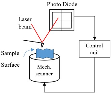
a)

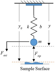
b)

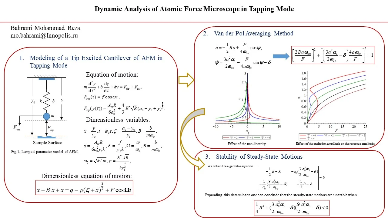
2. Modeling of a tip excited cantilever of AFM in tapping mode

This section covers the modeling of a tip excited AFM cantilever. To construct the model, we use the lumped model of the cantilever as shown in Fig. 1(b).

One can write the equation of the motion of the system, shown in Fig. 1(b), as:

where $m$ denoted to the effective mass of the cantilever located at the spring (massless) end. The stiffness and corresponding damping coefficient of the spring are designated by $k$ and $b$. The excitation force, $F_{ext}$, applies on the cantilever tip. There exists another force, sample surface-cantilever tip interaction force, acts on the tip. In this work, the DMT force is considered as this interaction force, $F_{tip}\left(y\right(\tau \left)\right)$.

These forces, $F_{ext}\left(\tau \right)$ and $F_{tip}\left(y\right(\tau \left)\right)$ are:

In Eq. (2), $f$ denotes to the amplitude of excitation, $\omega$ is the frequency of excitation, the Hamaker constant is shown by $A_H$, the tip apex radius is presented by $R$, $a_0$ is the inter-molecular distance, $E^{*}$ is the effective elastic modulus, and the fixed base frame coordinate distance to the sample is illustrated by $y_0$.

Substituting Eq. (2) in Eq. (1) we have:

To rewrite Eq. (3) in dimensionless format, we introduce dimensionless variables as:

where $y_s$ is the relax point of the static system, which can be get from Eq. (3) by putting the time terms and external excitation force, i.e. $f$ in Eq. (3) to zero, i.e.:

Substituting Eq. (4) in Eq. (3) one can write the dimensionless equation of motion as:

In this paper, dot denotes to derivation with respect to $t$.

3. Van der Pol averaging method

To solve Eq. (6), in this article, the Van der Pol averaging method is used. To use Van der Pol averaging method, first we need to approximate the DMT force around the equilibrium point $y_s$ as:

Defining new variables as:

one can rewrite Eq. (6) as:

where ${\omega }_{0n}=\sqrt{1-{\alpha }_1}$.

However, one can suppose that the external excitation frequency is near to the natural frequency of the oscillator, where the frequency difference $\mathrm{\Omega }={\omega }_{0n}+\delta$ is small. The detuning parameter, $\delta$, describes how near $\mathrm{\Omega }$ is to ${\omega }_{on}$. As one can mention from Eq. (8), the right-hand side terms are corresponding to dissipation, external excitation, and non-linearity. Since we assume they are small, it is advisable to construct the solution in the quasi-harmonic oscillation form with a slow changing amplitude, for which a shortened equation can be derived using asymptotic methods [16].

Expressing the solution of Eq. (8):

where $cc$ denotes to the conjugate part. An additional condition is introduced on the slowly changing complex amplitude $A$ [16]:

One can write the external force as:

First and second derivative of Eq. (9) with respect to time $t$ will be:

Now, by substituting Eqs. (9), (11) and (12) in (8), we have:

Times both sides of Eq. (13) by $\mathrm{e}\mathrm{x}\mathrm{p}-i{\omega }_{0n}t$, dividing by $i{\omega }_{0n}$ and averaging over the period of fluctuations, i.e. $2\pi /{\omega }_{0n}$, we obtain:

At this time scale, we disregard the change in complex amplitudes, and also the term containing the exponent since they change slowly. Then by omitting the rapidly oscillating terms, we come to a shortened Eq. (14).

The solution of Eq. (14) can be written in the form of:

where $a$ and $\beta$ are real variables.

Substituting Eq. (15) into (14), and separating the real and imaginary parts, we have:

Solving for $\dot{a}$ and $\dot{\beta }$, and introducing $\psi =\beta -\delta t$, we have:

Setting $\dot{a}=\dot{\psi }=0$ in Eq. (18), one obtains:

Squaring and summing equations in Eq. (19) leads to the frequency response:

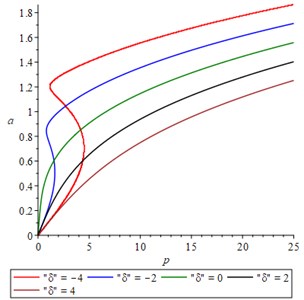
To investigate the effect of non-linearity and amplitude of excitation on the response we use Eq. (20). Results are shown in Fig. 2.

Eq. (20) shows that the maximum of the amplitude, $a_p=F/2{\omega }_{0n}B$, does not depend on the ${\alpha }_3$, the non-linearity. The non-linearity on the response amplitude is illustrated in Fig. 2(a).

Fig. 2a) Effect of the non-linearity, b) the excitation amplitude on the response amplitude for several detunings

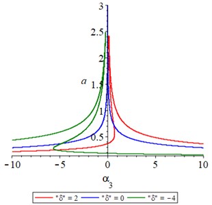
a)

b)

The effect of the excitation amplitude is shown in Fig. 2(b). As expected by increasing the amplitude of the excitation force increases the response amplitude. Also, depending on the value of $F$, some of the frequency-response curves are multivalued while others are single valued (Fig. 2(b)).

4. Stability of steady-state motions

To study the stability of the different portions of the response curves one can use different methods [17, 18].

To determine the stability of the steady-state motion by studying the singular points nature of Eq. (18), we set:

Substituting Eq. (21) into Eq. (18), expanding for small $a_1$ and ${\psi }_1$. It should be mentioned that $a_0$ and ${\psi }_0$ satisfy Eq. (19). Omitting nonlinear terms in $a_1$ and ${\psi }_1$, we get:

Accordingly, the steady-state motions stability depends on the eigenvalues of the right-hand sides coefficient matrix of Eq. (22). Then, we obtain the eigenvalue equation using Eq. (19):

Expanding this determinant one can conclude that the steady-state motions are unstable when:

and are otherwise stable.

5. Conclusions

The AFM is a valuable tool for imaging, measuring, and manipulating material at the nano-scale. The surface information is gathered by probing the surface with a mechanical scanner. The most precise scanning is done by using piezoelectric elements that facilitate small but accurate and precise movements on electronic command. The lumped parameter model has been used to construct the mathematical model of the tip excited AFM cantilever under the influence of DMT force. Because of the DMT force, the system became nonlinear. To solve the equation of motion, the Van der Pol averaging method has been used. The obtained frequency response equation has been utilized to examine the effect of non-linearity, and the excitation on the response. The stability of steady state motion has been studied.