Effect of excitation frequencies on phase contrast in tapping mode atomic force microscope

1. Introduction

Atomic force microscope (AFM) was invented in the 1980s [1] and is considered to be a versatile and powerful tool which can provide rich sample surface information, including friction, adhesion, topography, and viscoelasticity [2, 3]. The tapping mode AFM (TM-AFM) is able to obtain topographies and phase images simultaneously [4, 5]. Since the phase changes indicate the variations in the material property, materials with different damping characteristics will tend to lead to different phase offsets. Typically, the differences between the different phase offsets generated by points with different properties can be interpreted as the phase contrast [6]. The analysis of the contrast in the phase responses of TM-AFM is a powerful approach for the mapping of compositional variations in heterogeneous samples [7]. In addition, the in-plane structural and mechanical properties of the samples can be accurately revealed, [8] which are normally obscured in topographic imaging results [9].

The factors which affect the phase contrast in TM-AFM can mainly be divided into the following three categories: 1. Experimental environments; 2. Operating methods; and 3. Inherent properties of the AFM system [10-12]. A great deal of work has been conducted regarding the aforementioned factors in previous research in order to acquire phase images with high contrast. In regard to the experimental environments, the effects of air humidity [10] and ambient temperature [12] on the phase contrast have been studied in detail. Furthermore, regarding the operational approaches, the set point amplitude [11] and excitation values of the second normal mode of the micro cantilever [13] have been examined. For the inherent properties of the AFM, several researchers have proposed that energy loss, such as adhesion hysteresis and viscoelasticity, will affect phase contrast imaging [14]. Apart from the aforementioned investigations, the influencing effects of the AFM probe surface hydrophilicity have also been considered [10]. The geometric characteristics and sizes of the cantilevers have been investigated and compared [15].

In addition, it was well-known that a slight offset in the drive frequency effects the phase contrast and it was even implemented in many commercial systems. Some manuals (for example, MultiMode SPM Instruction Manual, NanoScope Software Version 5) have suggested that the system will work well in tapping mode if the drive frequency is at or below the peak level in the resonance plot. However, these understandings were mainly obtained through experiences, and there was no theoretical explanation of the underlying principles.

Therefore, the goal of the present research was to propose a simple theoretical model that demonstrates the effect of different excitation frequencies on the phase contrast. A theoretical formula between the phase contrast and excitation frequency was derived. In addition, in order to verify the above-mentioned hypothesis, sample with large differences in surface properties was selected for this study’s experiments. Furthermore, the contrast for all phase images was quantified in order to compare and optimize the excitation frequencies. The quantitative agreement between the theory and experimental results supported the correctness of the theoretical model.

2. Theoretical model

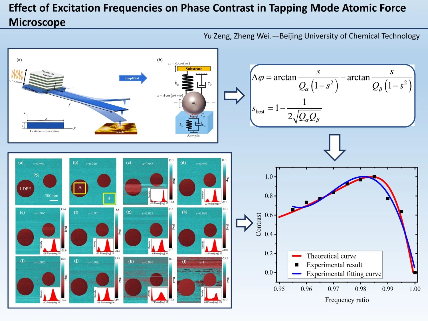
As shown in Fig. 1, the key component of TM-AFM is a microcantilever beam that is extremely sensitive to weak forces. In tapping mode, the microcantilever beam vibrates at or near its first-order natural frequency under the excitation of a piezoelectric actuator at its end [1]. The probe tip intermittently contacts the surface of the sample, and the vibration of the microcantilever beam is affected by the interaction force between the tip and the sample surface. By attaching a laser beam and a photodetector to the probe surface, the vibration signal of the free end of the probe can be measured, and the phase image of the sample surface can be obtained. In Fig. 1, $l$, $b$, and $d$ denote the length, width, and thickness of the cantilever beam, respectively, and the vibration equation of the microcantilever beam under the tip-sample force is:

where $u$ represents the absolute displacement of the microcantilever beam, $E$ and $I$ are the Young’s modulus and the moment of inertia of the cross-section of the microcantilever beam respectively, $\rho$ is the density of the microcantilever beam, $c$ represents the damping per unit length of the microcantilever, $F_{ts}$ represents the interaction force between the tip and the sample, and $\delta \left(x-l\right)$ is the Dirac function.

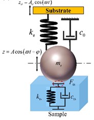
Fig. 1a) Schematic diagram of the vibration of the tapping atomic force microscope probe; b) schematic diagram of one-dimensional mass-spring-damping vibration model

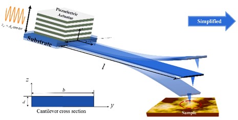
a)

b)

In TM-AFM, the piezoelectric actuator at the fixed end of the microcantilever beam drives the microcantilever beam by support excitation. The support excitation is represented by $z_d=A_d\mathrm{s}\mathrm{i}\mathrm{n}\varpi t$, where $A_d$ is the excitation amplitude and $\varpi$ is the excitation frequency. Typically, TM-AFM probes vibrate near their first natural frequency, and surface information of the sample is obtained by monitoring the displacement of the tip. When vibrating at the first natural frequency, the steady-state response of the free end of the microcantilever is harmonic, consistent with the vibration solution of a single-degree-of-freedom spring-mass system. Therefore, the microcantilever model can be simplified to the spring-mass model as depicted in Fig. 1(b). The equation of motion for the motion of the free end of the microcantilever subjected to support excitation at or near the first natural frequency can be represented as follows:

where $m_e$ represents the equivalent mass of the microcantilever beam; $c_0$ represents the equivalent external damping that describes background dissipation; $k_e$ is the spring constant of the microcantilever beam;$z$ represents the absolute displacement of the tip; and $z_d$ represents the support excitation. A number of studies have now shown that the tip-sample contact stiffness is small and has little effect on the intrinsic frequency of the probe [5, 16, 17]. Therefore, the effect of $k_{ts}$ can be neglected and Eq. (2) can be simplified as:

where ${\omega }_0$ is the first order intrinsic frequency of the system; $Q$ denotes the total quality factor of the system. In this paper, the quality factor denotes the ratio of the total energy to the dissipated energy in one vibration cycle of the microcantilever beam, and $Q$ can be expressed by the following equation:

where $W$ represents the total energy of the system during one oscillation period, while $W_0$ represents the dissipated energy of the system during one oscillation period. From Eq. (3) we get the expression for the phase as:

where $s=\varpi /{\omega }_0$ represents the ratio of the excitation frequency to the natural frequency. In TM in AFM, phase images are obtained by monitoring the phase deviation of the probe at various positions on the sample surface. The phase deviation between two different components on the sample surface is called the phase difference, which reflects the difference in the physical and chemical properties of the two components. In the present investigation, for convenience purposes, the damping of the two scanned areas were referred to as $Q_{\alpha }$ and $Q_{\beta }$, respectively. Therefore, it could be assumed that ${\phi }_{\alpha }$ and ${\phi }_{\beta }$ represented the phase offsets on the surface regions corresponding to $Q_{\alpha }$ and $Q_{\beta }$, respectively. Subsequently, from Eq. (5), the phase contrast $\mathrm{\Delta }\phi$ was written as:

where $Q_{\alpha }$ and $Q_{\beta }$ represent the dissipation quality factors of the AFM probe tip when it is located in regions with different properties on the sample. From Eq. (6), it can be observed that phase contrast is directly related to the frequency ratio. Next, we will investigate the influence on contrast from excitation frequency and explore strategies for optimizing phase contrast.

3. Experiments

The excitation frequency of the piezo actuator is one of the most fundamental and easily adjustable parameters in the operation of the TM-AFM. From Eq. (6), it can be seen that the phase contrast depends only on the excitation frequency when two microcantilever systems operate in different characteristic regions. By taking the first-order derivative of Eq. (6) and taking the value of its first-order derivative to be zero, the optimum value of Eq. (6), that is, the optimum excitation frequency corresponding to the maximum phase difference, can be obtained with the value of:

Since in typical situations, the magnitude of quality factors ranges from tens to hundreds, thus $Q_{\alpha }{Q}_{\beta }\gg 1$ is greater than 1. Therefore, expanding through Taylor series, the above equation can be simplified to:

From Eq. (8), it can be observed that theoretically, there exists an excitation frequency to maximize the phase contrast. This theoretically explains why, during experiments, when less than ideal phase images are obtained, experimenters often fine-tune the excitation frequency to be slightly below the first natural frequency to achieve more ideal phase contrast images.

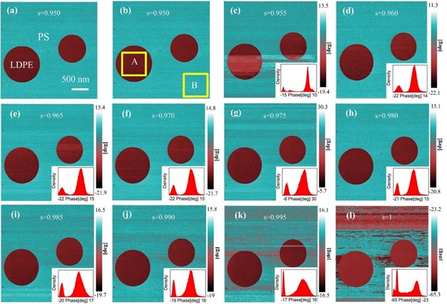
The experiments were performed using a Bruker DIMENSION XR AFM. The type of probe used in the experiment was a Tap AN-NSC10 probe. All of the measurements were performed under room temperature conditions and at a relative humidity of approximately 30 %. Large free-oscillation amplitudes were chosen in order to ensure that the probe would not be captured by the sample surface. In accordance with the frequency sweeping curves, it was determined that the natural frequency of the system was 188.756 KHz. When the excitation frequency was greater than the natural frequency of the system, the sign of the phase offset would change, which increased the difficulty of analyzing the experimental results. Therefore, the excitation frequency was selected to the left of the system natural frequency in this study. For the PS-LDPE sample, ten sets of experiments were conducted near the resonance frequency. During the experiments, the excitation frequency ratio was gradually increased from 0.955 until the excitation frequency ratio reached 1.000. The phase images obtained from this study’s experiments are shown in Fig. 2.

As revealed in Fig. 2(a), there were obvious features observed. For example, it can be seen in the figure that the LDPE is located in a reddish-brown circular area, while the PS is placed in a light green background area. Phase images are depicted in Figs. 2(c-l) for 10 frequency ratios ranging from 0.955 to 1.000, respectively. It was clearly seen by simple observation that the phase images contained horizontal stripes with opposite contrast or irregular wavy features [Fig. 2(c) and Figs. 2(k-l)]. Their appearance was most probably due to the improper selection of the excitation frequency. This was also the reason why the excitation frequency was not taken at the resonance frequency. In order to further distinguish the contrast, the phase distributions of the images were taken into consideration. The corresponding histogram was observed to have two peaks related to the PS and LDPE [insets in Figs. 2(c-l)]. In the histograms, the abscissa represents the phase, and the ordinate represents the density of the phase within the entire image. It can be seen that Figs. 2(d-j) all exhibit clear contrast. However, their phase images are very similar to each other, and their histograms all have two peaks. Therefore, it was not clear which image had the best contrast, and the corresponding excitation frequency could not be confirmed. Therefore, a quantitative study was necessary.

Ideally, PS-LDPE is composed of two components which correspond to two single lines in the histograms. The two peaks which appeared in this study’s histograms were due to the fact that the sample did not have ideal purity and the influence of experimental operation. Each peak was expressed by a Gaussian distribution. This study gathered the data in Squares A and B [Fig. 2(b)], which represented the phase distributions of the LDPE and PS, respectively. The sizes of A and B were both 1.1 μm×1.1 μm. The larger the areas of A and B were, the closer the experimental values would be to the true values. The locations of the data points gathered in Figs. 2(c-l) were the same as those shown in Fig. 2(b). In order to quantify the phase contrast, Ashman’s $D$ was introduced, which was derived by the following statistical formula [18]:

where ${\mu }_1$ and ${\mu }_2$ are the means of the phases of the data points in Squares A and B, respectively, and ${\sigma }_1$ and ${\sigma }_2$ represent the standard deviations. Each image has a specific $D$ in Figs. 3(c-l). A larger $D$ indicates a better contrast result. Therefore, by referring to $D$, the image with the best contrast could be easily determined.

Fig. 2Experimental phase images of PS-LDPE: a) scanning phase image of PS-LDPE, in which the total scan size was 4.5 μm×4.5 μm; b) the areas enclosed by the yellow squares are the value areas of the processed experimental data, in which Area A corresponds to the LDPE, and Area B corresponds to the PS; c)-n) Phase images and corresponding histograms for 10 groups of frequency ratios from 0.955 to 1.000, where s is the frequency ratio

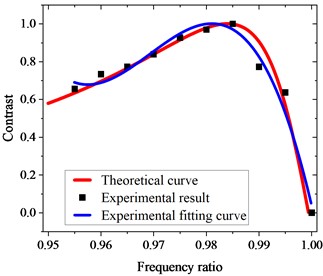
We assume that $D^{*}=\mathrm{\Delta }{\phi }^{*}$, where $D^{*}$ and $\mathrm{\Delta }{\phi }^{*}$ are the normalized $D$ and $\mathrm{\Delta }\phi$, respectively. In total, there are 10 sets of experimental results, which means there are 10 sets of solutions. When most of the solutions satisfy the relationship $D^{*}=\mathrm{\Delta }{\phi }^{*}$, the fit yields $Q_{\alpha }=\text{18}$ and $Q_{\beta }=\text{54}$. They represent the total quality factor of the system when the tip is in contact with PS and LDPE, respectively. The smaller the value of $Q$, the greater the energy dissipation. That is to say, the damping of the PS surface is greater than that of LDPE. In this study, after determining the values of $Q_{\alpha }$ and $Q_{\beta }$, the corresponding theoretical curves can be obtained by using Eq. (6), and the experimental results and the theoretical curves were successfully plotted after normalization, as shown in Fig. 3.

The experimental results were found to be highly consistent with the theoretical results. This was possibly due to the fact that there were hundreds of data points located in Squares A and B. Calculating the means and standard deviations of the phases of hundreds of points can effectively eliminate the errors caused by the experimental operations. As a result, the calculated phases were very close to the true phases. This also confirmed that it was feasible to use Eq. (6) to describe phase contrast and to obtain the best excitation frequency range. Substituting $Q_{\alpha }$ and $Q_{\beta }$ into Eq. (8), the theoretical optimal frequency ratio is obtained to be 0.984. And the experimental results also show that the phase contrast of two different nature regions reaches the maximum when $s\approx$ 0.985, which is almost exactly consistent with the theoretical results.

Fig. 3Theoretical curve and experimental results of the PS-LDPE sample

Based on the above results, in the experiment, we can get the optimal excitation frequency by the following methods. Firstly, the excitation frequency near the intrinsic frequency of the system is selected to scan the sample, and then the experimental results are fitted by Eq. (6) to obtain the total quality factors $Q_{\alpha }$ and $Q_{\beta }$ when the tip of the needle touches the two different components in the sample respectively. The optimal excitation frequency for phase imaging of a two-phase mixture can then be obtained theoretically by using Eq. (8), and the phase image with optimal phase contrast can be obtained by scanning with this optimal excitation frequency.

4. Conclusions

In this article the effect of different excitation frequencies on phase contrast in the tapping modes of AFM were examined. A theoretical formula between the phase contrast and the excitation frequency was successfully derived. In addition, PS-LDPE samples were selected for the experimental processes. The quantitative agreements between the theoretical and experimental results verified that the excitation frequency will affect the phase contrast. The best excitation frequency of PS-LDPE is around 184 KHz and the optimal excitation frequency is slightly smaller than the resonance frequency. The phase contrast was observed to worsen when the drive frequency approached the resonant frequency. In addition, both theory and experiment have demonstrated that there exists an optimal excitation frequency that maximizes the phase contrast during the scanning process. Therefore, using this optimal excitation frequency in the experiments, the best phase image with the best contrast can be obtained. This is important for interpreting the phase image and guiding the experiments.