The control of a five-axis robotic arm and its experimental application

1. Introduction

In this study, the control of a five-axis robotic arm, including computation of its orbit, has been achieved. The MATLAB 2010a (student edition) and LabVIEW 2010 (student edition) applications have been used to perform the computations. A PC expansion card, manufactured by JS Automation (part number AIO-3320) and having LabVIEW support, has been used to communicate with the robotic arm through the PCI port. The values obtained through the inverse kinematics computations performed using the LabVIEW and MATLAB applications have been relayed to the robotic arm over the AIO-3320 expansion card, using LabVIEW [1].

2. Problem statement

The analytical calculation method has been chosen for use when performing forward and inverses kinematics computations. The robotic arm is rotated using servo motors. LabVIEW, a graphical programming environment, has been used as the programming language. The LabVIEW system was chosen for its capability for parallel computation. It has been possible to simultaneously operate more than one servo motor with this parallel operation capability. Additionally, LabVIEW provides support to run MATLAB scripts and functions. (This requires MATLAB to be installed on the PC along with LabVIEW.)

MATLAB has been used for analytical calculations, for matrix operations (e.g. matrix multiplication, finding inverses), and for solving non-linear equations.

2.1. Forward kinematics computations for the robotic arm

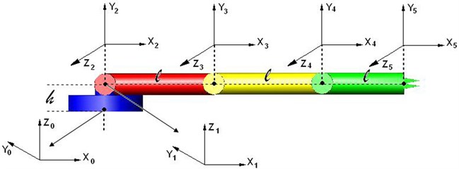
The Denavit-Hartenberg method has been used to obtain the forward kinematics models. As shown in Fig. 2, joint variables and constants are defined using the Denavit-Hartenberg method and the coordinate systems are placed over the joints. [2]

Fig. 1The robotic arm used in the study

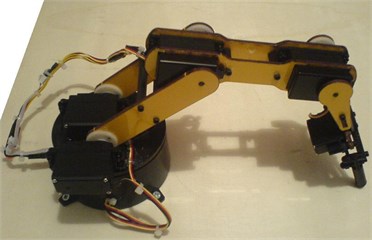
Fig. 2Coordinate frames of the robotic arm with four degrees of freedom

The Denavit-Hartenberg variables are shown in Table 1. The parameters which do not change as a result of the motion of the robot are the length of the arm $a_{i-1}$, and the angles of the axis ${\alpha }_{i-1}$. The parameters that vary are the joint angle ${\theta }_i$ (in case of a rotating joint), and the joint offset $d_i$ (in case of a prismatic joint) [3].

The homogenous conversion matrix for the arm is shown below, where $i$ is the axis number.

Table 1D-H variables

Axis number	D-H variables				Joint variable
$i$	${\alpha }_{i-1}$	$a_{i-1}$	$d_i$	${\theta }_i$	$d_i$ or ${\theta }_i$
1	0	0	h	${\theta }_1$	${\theta }_1$
2	90	0	0	${\theta }_2$	${\theta }_2$
3	0	l	0	${\theta }_3$	${\theta }_3$
4	0	0	0	${\theta }_4$	${\theta }_4$
5	0	0	0	${\theta }_5$	${\theta }_5$

$s_i=\sin {\theta }_i$ and $c_i=\cos {\theta }_i$. ${\theta }_i$ is the rotation angle and:

1

${}^0{\mathbf{T}}_5=\left[\begin{array}{cc}{{}^{0}R}_5& {{}^{0}p}_5\\ 0& 1\end{array}\right]=\left[\begin{array}{cccc}{r}_{11}& r_{12}& r_{13}& p_x\\ r_{21}& r_{22}& r_{23}& p_y\\ r_{31}& r_{32}& r_{33}& p_z\\ 0& 0& 0& 1\end{array}\right].$

${{}^{0}R}_5$ is the rotation matrix and ${{}^{0}p}_5$ is the position vector. The transformation matrices for the first and the second joint are:

2

${{}^0\mathbf{T}}_{1=}\left[\begin{array}{cccc}{c}_1& -s_1& 0& 0\\ s_1& c_1& 0& 0\\ 0& 0& 1& h\\ 0& 0& 0& 1\end{array}\right],{{}^1\mathbf{T}}_{2=}\left[\begin{array}{cccc}{c}_2& -s_2& 0& 0\\ 0& 0& -1& 0\\ s_2& c_2& 0& 0\\ 0& 0& 0& 1\end{array}\right].$

The transformation matrix for the third, fourth, and fifth joints is:

3

${{}^{i-1}\mathbf{T}}_i=\left[\begin{array}{cccc}{c}_i& -s_i& 0& l\\ s_i& c_i& 0& 0\\ 0& 0& 1& 0\\ 0& 0& 0& 1\end{array}\right].$

The five transformation matrices that have been computed are multiplied to obtain the rotational matrix for the arm:

4

${{}^0\mathbf{T}}_5={{}^0\mathbf{T}}_1{{}^1\mathbf{T}}_2{{}^2\mathbf{T}}_3{{}^3\mathbf{T}}_4{{}^4\mathbf{T}}_5.$

The transformation matrices obtained through Eq. (1) and (4) are equivalent.

3. Result and discussion

We will use forward kinematics Eqs. (1) and (4) for computations Eq. (1) and (4) are equal to each other. By multiplying each side of the Eq. (4) with the inverse of ${{}^0\mathbf{T}}_1$, we obtain the Eq. (5).

Since ${{{}^0\mathbf{T}}_1^{-1}{}^0\mathbf{T}}_5={{{}^0\mathbf{T}}_1^{-1}{}^0\mathbf{T}}_1{{}^1\mathbf{T}}_2{{}^2\mathbf{T}}_3{{}^3\mathbf{T}}_4{{}^4\mathbf{T}}_5$ and ${{}^{i-1}\mathbf{T}}_i^{-1}.{}^{i-1}{\mathbf{T}}_i=\mathbf{I}$, it follows that:

Let’s find the inverse matrices for all transformational matrices in Eq. (2) and Eq. (3), using the inv() function in MATLAB [4]:

The position vectors located within Eq. (5) are mutually equalized and the following equations are then obtained:

Let’s label the left-hand side of Eq. (7) as $A$:

Similarly, let’s label the left-hand side of Eq. (9) as $B$:

Each side of Eq. (5) is multiplied with ${{}^{1}T}_2^{-1}$:

In Eq. (12), the position vectors are equalized and the equations below are obtained:

Each side of Eq. (12) is multiplied with ${{}^{2}T}_3^{-1}$:

The position vectors in Eq. (15) are equalized, and the following equations are obtained:

In the inverse kinematics solution, the angle ${\theta }_1$ is solved from Eq. (8). The angles ${\theta }_2$, ${\theta }_3$ and ${\theta }_4$, on the other hand, are obtained through iterations. For the three unknowns, Eqs. (13, 14, 17) have been selected. The ${\theta }_5$ the angle indicates the open and close states of the end effector. This angle does not affect the position vector but affects only the rotation matrix.

3.3. 3.2.1. Orbit planning using LabVIEW

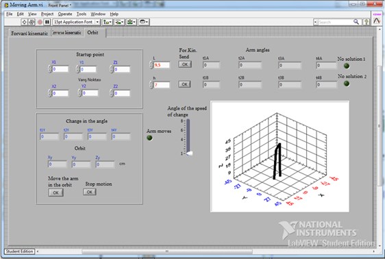
The code moves the robotic arm from its starting position coordinate of ($X1$, $Y1$, $Z1$) to its ending position coordinate of ($X2$, $Y2$, $Z2$). Fig. 3 shows the corresponding user interface.

3.3.1. Outline for the orbit computation algorithm

1) Using the inverse-kinematic.vi function, compute the angles necessary for the starting position coordinate (Fig. 4).

2) Using inverse-kinematic3.vi, correct the computed angles.

3) Using the inverse-kinematic.vi function, compute the angles necessary for the ending position coordinate.

4) Using inverse-kinematic3.vi, correct the computed angles.

5) If steps 1, 2, 3 and 4 produce a solution and if the “Move arm along the orbit” box has been clicked:

a) Find the difference between t1A and t1B, convert it into the digital value required by the robotic arm, and bind the value to the “Difference of t1A and t1B” indicator.

b) Bind the state where t1A is larger than t1B to the “t1A > t1B” indicator.

c) Repeat steps a and b for remaining angles.

6) Illustrate a for loop running from 0 to 16384.

7) Within the for loop:

a) Use $i$, the loop variable, as the numeric value for the angle of the robotic arm.

b) Determine angle value as i_say = i_say + “rate of change of the angle”.

c) If the “t1A>t1B” indicator value is “true”, increment the numerical value of the t1A angle by the value of i_say; if “false”, decrement it by the value of i_say.

d) Convert the value in step c into degrees and bind it to the t1Y control.

e) Repeat steps a, b, c ,and d for remaining angles.

f) When the “t1A t1B” value and the corresponding values for the remaining angles are less than the value of i_say, or when the “arm is moving” indicator light is off, exit the loop.

g) Move the arm to the position indicated by t1Y and the remaining angles.

Table 2Functions used in orbit planning [6]

Name of function	Symbol	Description
T01.vi		Creates transformation matrix using height (-$h$), arm length (-$L$), and angle values.
forward-kinematic.vi		Creates transformation matrixes from the start to the end positions, and vectors PX, PY and PZ, based on the transformation matrix.
inverse-kinematic.vi		Computes the angles t2, t3 and t4 as well as other items from coordinates $X$, $Y$, and $Z$.
inverse-kinematic3.vi		Moves angles computed by the inverse-kinematic.vi function into arm boundaries.
aio3320_signal_transformation.vi		Converts an angle value in degrees to analog/digital signals or converts analog/digital signals into an angle value in degrees.

Fig. 3The user interface showing the “Orbit” tab

3.3.2. LabVIEW diagrams for the “Orbit” tab

Fig. 5 shows the calculation of the starting and ending angles using the “inversekinematic.vi” function. The output contains indicators t1A, t1B, t2A1, t2B1, t3A1, t3B1, t4A1, and t4B1.

Fig. 4The LabVIEW code for “inversekinematic.vi” making use of MATLAB

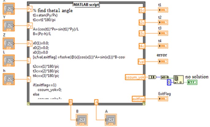
Fig. 5Calculation of the starting and ending angles using the inversekinematic.vi function

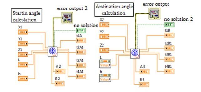
Fig. 6Correction of the starting and ending angles

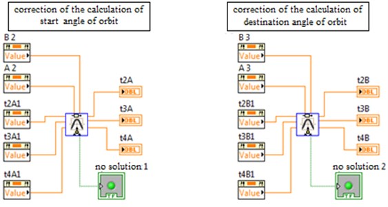
Figs. 6 show corrections applied to the angles computed in Fig. 5, using the inversekinematic3.vi function. Angle t2A1 is transformed to t2A, angle t3A1 to t3A, and angle t4A1 to t4A; the same applies to t2B, t3B, and t4B. For the computation of the orbit, the angle ${\theta }_1$ of the robotic arm will change from t1A to t1B, the angle ${\theta }_2$ from t2A to t2B, the angle ${\theta }_3$ from t3A to t3B, and angle ${\theta }_4$ from t4A to t4B. The change of the angles from A to B is accomplished using a for loop shown in Fig. 7.

Fig. 7The program for-loop [7, 8]

The for-loop shown in Fig. 7 is located in a case structure having the conditions shown in Fig. 8. To move the arm, the angles of the positions A and B must be calculated, the “No Solution” indicator light must be off, and the “Move arm along the orbit” button must be clicked.

Fig. 8Condition for the robotic arm movement within the “Orbit” tab

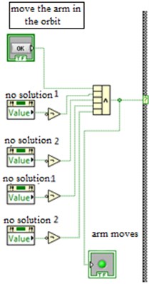
Fig. 9Determining the differences of the angles for positions A and B, and whether they are large or small

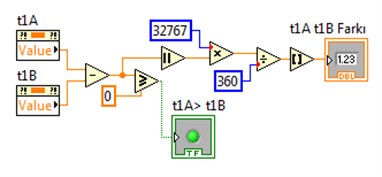
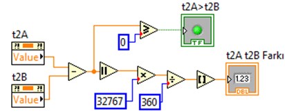
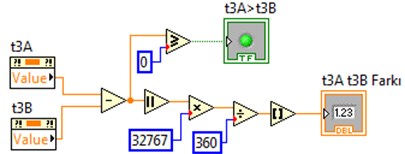
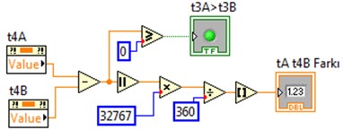
Fig. 9 shows the differences between the angles for position A and the angles for position B having been converted into the digital values required by the arm. Additionally, for each angle, a boolean indicator has been used to indicate whether the movement from A to B will be in increasing or decreasing terms. If angle A is larger than angle B, this indicator is set to true; otherwise, the indicator is set to false.

3.3.2.1. Diagrams within the for loop

The transition of the arm from position A to position B is accomplished using for a loop.

For the angles to get closer to position B from position A, on each iteration through the loop, the angles are adjusted by the value contained in i_say. The for loop variable $i$ is at value zero at the start of the for a loop. For each iteration of the loop, its value is incremented by 1. It runs if the condition of the case structure shown in Fig. 10 is “true”. It sets the i_say indicator value to zero. In Fig. 10, the value contained within “The angle rate of change” control is added to the value of i_say, and its output is assigned to i_say.

Fig. 10Definition of angle increment and decrement values within the for loop

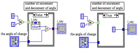
Fig. 11Conditions for an early exit from the for loop

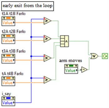
In the program code shown in Fig. 11, the value of the i_say indicator is continuously incremented. When the value of i_say is larger than the difference of the angles for position A and position B, the loop is exited. This means that the arm has arrived at position B.

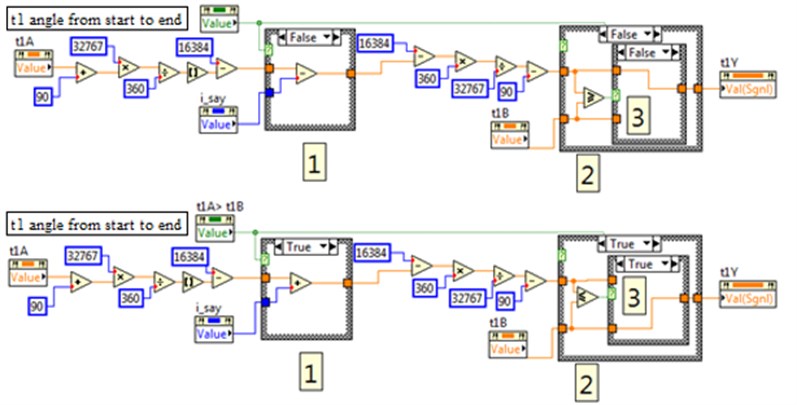
We will now describe the block diagrams shown in Fig. 12. The condition for the case structure shown in (1) is the “t1A > t1B” indicator. If this value is “true”, the approach from the t1A value to t1B value is in increments of i_say; otherwise, if the value is “false”, the approach is in decrements. The values are converted to degrees using mathematical processing at the output the of case (1). This value goes to t1Y value until it arrives at t1B value. When it reaches t1B, it goes to the value of t1Y. Fig. 12(a) and 12(b), and Fig. 12(c) and 12(d) are sequential. A Similar method is applied for angles t2, t3, and t4.

Fig. 12Code that moves angle t1 from position t1A to position t1B

4. Conclusions

Forward and inverse kinematics computations have been performed using LabVIEW and MATLAB. Transformation matrices and their multiplication have been employed in the computations. Using the software developed, the required end coordinate ($X$, $Y$, $Z$) for the robotic arm is provided. The study has been implemented on a robotic arm, and it has been observed that the arm has moved to the position indicated by the $x$, $y$, and $z$ values entered. Following the entry of two coordinates into the system, the arm has first located to the starting position and then moved to the ending position. Throughout the movement of the arm along the orbit, the current coordinate computed by the software is displayed by the user interface.

The study has met its objective. Using the software, the movement of the end effector between two positions has been accomplished. With minor modifications in the software, the arm can be made to visit more than one position along the orbit.

During orbit planning, it has been assumed that no obstacles exist which would affect the orbit.