Abstract
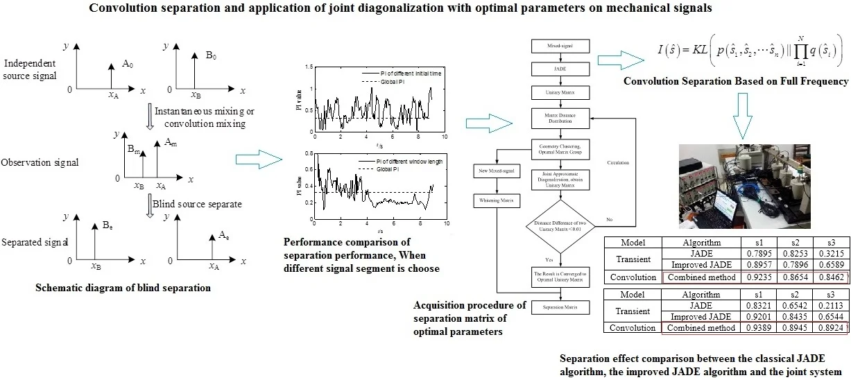
Blind separation algorithm has the problem of separation stability in the condition of multiple convolution signals. Based on cluster analysis, combined with the optimal distance matrix and the optimal window, the joint diagonalization is improved, which can effectively improve the stability and accuracy of the signal separation. The full frequency divergence is set as the objective function of permutation ambiguity in the convolution separating process, the failure from convoluted blind source separation is solved. Combining with new joint diagonalization and convolution separation is to form a system approach, and is applied to the floor signal from the actual bench, the influence of excitation source in frequency is achieved, the system algorithm can be used as a reference of mechanical vibration analysis.
Highlights
- Based on cluster analysis, combined with the optimal distance matrix and the optimal window, the joint diagonalization is improved, which can effectively improve the stability and accuracy of the signal separation.
- The full frequency divergence is set as the objective function of permutation ambiguity in convolution separating process, the failure from convoluted blind source separation is solved.
- Combining with new joint diagonalization and convolution separation is to form a system approach, and is applied to the floor signal from the actual bench, the influence of excitation source in frequency is achieved.
1. Introduction
The influence factors of vehicle vibration or noise, such as automobile’s diversified running condition and coupling characteristics of excitation source, are complex. Blind Source Separation, as a high-order digital processing method, can obtain the characteristics of excitation source relatively quickly and easily. However, the choice of algorithms and the practical application face more uncertainties, which will affect the accuracy of the results.
At present, there are many blind separation algorithms in mechanical field, based on object compound degree, which are divided into instantaneous mixing algorithm and convolution algorithm, such as FastICA (Fast Independent Component Analysis), Jade (Joint Approximative Diagonalization of Eigenmatrix), Sobi (Second Order Blind Identification), Sons (Second Order Non-stationary Source Separation), Cmjd (complex matrix joint diagonalization), JBD (Joint Block Diagonalization), etc [1-6]. Convolution algorithms have time-domain algorithm, which based on second-order statistics, high-order statistics and information theory, and the application of instantaneous blind separation in frequency domain convolution [7-9]. Most of the algorithms are transplanted directly from the field of speech communication to the field of mechanical signals. Different from the voice transmission, the mechanical structure has limited transmission paths, and has variety of frequency response characteristics, resulting in the separation instability of the algorithm.
In this paper, the joint diagonalization algorithm with definite physical meaning is taken as the object to discuss the influence of the window length and the starting parameter of the diagonalizable matrix. Utilizing European Geometric Clustering Analysis as the Optimum Parameter Acquisition Means to Realize the Stability and Accuracy Improvement of Instantaneous Separation Algorithm. Combined full-range divergence as the objective function of convolutional ambiguity arrangement, simplifying the acquisition of filter parameters, achieving the mechanical structure convolution signal blind separation, to apply to the stationary or non-stationary mixed mechanical signals.
2. Joint approximate diagonalization theory and blind separation performance evaluation
2.1. Joint diagonalization based on second-order correlation matrix [10]
Blind source separation (BSS) algorithm can directly separate the frequency domain characteristics of the source signal from the observed signal without knowing the system and source signal, and then separate the corresponding responses of different sources, so as to obtain the contribution of different sources in the response.
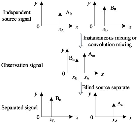
In the near source measurement, as shown in Fig. 1, the source signals are mixed in a certain way and separated based on BSS. This figure reflects that the blind separation method has the uncertainty of separation order and amplitude.
Fig. 1Schematic diagram of blind separation
The algorithm first obtains the whitened observation matrix of the observation signal, and then generates the higher order cumulant matrix, which can be diagonalized. The observation vector containing noise is treated as follows:
In the formula, the is the whitening matrix, is an independent source signal, is a mixed matrix, is a random noise matrix.
The whitened observation signal is the product of the source signal and the unitary matrix , and transforming from estimating to the determination of . The whitening matrix is obtained by the characteristic decomposition of the zero-delay variance of the observed vector, see Eq. (2):
In the formula, and are the eigenvalue matrix and eigenvector matrix corresponding to the zero-delay variance matrix of the observation vector respectively.
Since the cumulative amount of white noise is calculated as 0, based on Eq. (1), the delay correlation matrix of the whitened signal can be written as:
Under the assumption that the statistical independence of source signals is satisfied, in Eq. (3) is a diagonal matrix. Which means that the covariance matrix at different delay moments of can be diagonalized, that is:
By the diagonalization of the correlation matrix of the observed signals of all delay points, the cost function is the non diagonal element and the minimum of all the unitary elements, and then the unitary matrix :
The JADE algorithm based on second order blind identification (SOBI) and fourth-order blind identification (FOBI) has good numerical stability [11]-[14]. In most applications, especially in mechanical fault diagnosis, information is often included in the waveform of the signal. So, to some extent, the JADE algorithm based on the joint approximate diagonalization of the matrix can be applied to the instantaneous separation of the actual statistical correlation sources.
2.2. Separation effect evaluation index
In addition to the similarity coefficients and the quadratic residuals of the estimated signal and the source signal, since the separation matrix and the hybrid matrix are theoretically inverse matrices, it is possible to obtain a more accurate evaluation of the blind source separation algorithm by taking the separation matrix as the basis. A common index for evaluating the performance of blind separation is the PI (Performance Index), which is measured by the difference between the hybrid matrix and the separation matrix. Its definition [15] is as follows:
In the formula, is the global matrix, the product of the separation matrix and the mixing matrix , and is the th element of the matrix . Here, The smaller the value, the better the separation effect.
3. Joint diagonalization problem
Joint approximate diagonalization principle is to compare the different delay covariance matrix or higher order cumulant non diagonal square sum. When the time delay is larger, the number of delay matrix increases, and the relative separation accuracy will be improved a certain degree. But the matrix with large amount of time delay will have less effective data which use mixed signal. That is, the delay increased, which delay matrix correlation smaller, the use of uniform orthogonal matrix to diagonalization, the separation error will be a corresponding increase. The simulation signal Eq. (7) is used as the object of study, which is characterized in that the independent source signal contains noise (random noise) and contains non-stationary signal components. To study the relationship between the diagonalization blind signal separation method and the signal structure. The signal time is 10 s and the mixing matrix is randomly generated, [0.32 –0.43; –1.31 0.34]:
Fig. 2Performance comparison of separation performance, when different signal segment is choose
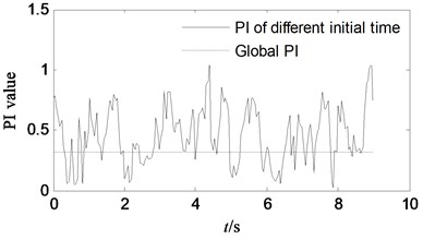
a) Separation performance PI curves of observed signal when choosing different initial time
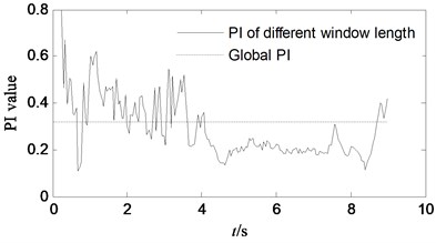
b) Separation performance PI curves of observed signal when choosing different window length
The relationship between the separation effect and signal structure of the joint diagonalization algorithm is studied from two perspectives. (1) to determine the starting point of the global signal, change the window length to achieve different algorithm identification; (2) to determine the window length of the intercept signal, change the starting point of different windows to achieve algorithm identification. Fig. 2 shows the performance comparison of different windows and starting points. It shows that there are some separation performance (the optimal starting point PI is 0.0296 and the optimal window PI is 0.1059) when choosing different starting time and window length, which is much better than that the PI based on global signal segment (0.3219). The effect of the start time and the window length on the separation effect is reciprocal. That is, the performance of the joint diagonalization algorithm in the case of noise or when the signal-to-noise ratio is poor (including non-stationary signals) is related to the window length and the starting time. The results show that when the data volume of the stochastic stationary signal is large, the whole data joint diagonalization, and the calculation amount is large, and the optimal separation effect cannot be always obtained.
The algorithm is applied to the signal from different starting points and different windows, and its essence is to obtain diagonalization matrix of different clusters, so as to obtain different separation effects [16]. For the original mixed signal, there should be a cluster of the best diagonalization of the matrix group, you can get the best separation effect. In Section 1, the joint approximate diagonalization method is the least square sum of the non-diagonal elements, caused by the matrix , as the cost function. Here, defining the square sum of the nondiagonal elements of the matrix, which distance is :
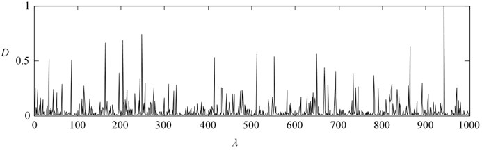
As shown in Fig. 3, matrix distance (distance normalization) under different delay matrices is obtained by matrix calculated with classical joint diagonalization algorithm. It is shown that the matrix distance has some randomness when the amount of delay increases, that is, it is not always possible to obtain the minimum value of Eq. (5) by using the unified matrix.
Fig. 3Matrix distance distribution of U matrix at different delay, when using classical JADE algorithm
4. Joint approximate diagonalization separation of optimal parameters
Based on the classical JADE method, the clustering is realized based on the array of matrix distance. A cluster diagonalization matrix near the center of the cluster is taken as the joint diagonalization unitary matrix. The new unitary matrix again calculates the matrix distance until the difference between the matrix distance, caused by this unitary matrix, and last time is less than the set value. That is, the iterative algorithm converges to the optimum, so as to obtain the optimal unitary matrix, and then get the optimal separation effect. The specific flow of the algorithm is shown in Fig. 4.
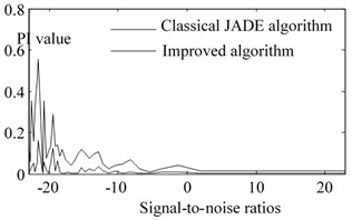
Take the source signal of Eq. (7) as an example, Fig. 5 shows the change of PI value during the iteration. It shows that when the new algorithm is iterated to 20 times, the PI value has reached 0.05, improving the accuracy of the original global diagonalization algorithm by more than 80 %. After applying the above algorithm, the separation performance can be improved. Fig. 6. shows the change of PI value in different random mixing matrix . Fig. 7 shows the application of the new algorithm under different signal-to-noise ratios. Compared with the classical JADE algorithm, in the low SNR stage, the improved diagonalization algorithm can effectively improve the accuracy. In the high SNR stage, the accuracy improvement effect is relatively small.
To sum up, through the different mixing matrix, different SNR and other types of state, validating that the new algorithm can effectively improve the precision and stability of separation.
Fig. 4Acquisition procedure of separation matrix of optimal parameters matrix diagonalization
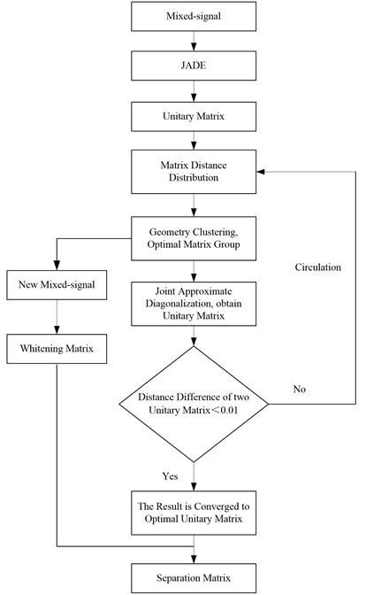
Fig. 5The change of PI value during the iteration
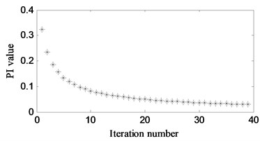
Fig. 6The change of PI value in different random mixing matrix A
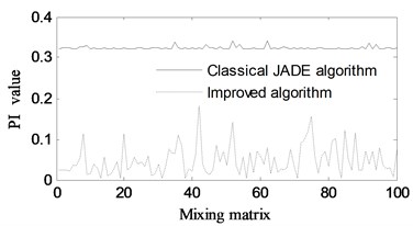
Fig. 7The change of PI value different s2 under signal-to-noise ratios
5. Convolution separation based on full frequency
In the convolutional mixing process, each frequency band can be regarded as an instantaneous mixing process [17]. There exists a separation matrix ( is the estimated source number, is the observed signal number), making the estimation sources independent of each other at the -frequency ( is the number of frames of the short-time Fourier transform).In the frequency domain, Eq. (9):
Similar to the instantaneous algorithm, different sources have independent features in each frequency band, and mutual information is used as the independent judgment between the frequency vectors, so that the cost function includes all frequency bands:
Formula,, , is the entropy of the observation vector, independent from the unmixing matrix , and can be discarded. Mutual information preserves the correlation of different frequency vectors in the same source in the cost function.
6. Application of convolutional blind separation for optimal parameter joint approximate diagonalization
In order to achieve the algorithmic application of the mechanical signal, combined optimal parameter joint diagonalization with frequency domain convolutional separation, based on the flow chart 3, which improving the joint approximation diagonalization for separation at the characteristic frequency point. Based on the ambiguity of mutual information correction frequency band arrangement, blind separation of hybrid mechanical signals is realized.
Setting general cantilever beam as the object, existing three excitation sources, the excitation source uses a number of signal generator as the output of the vibration. Unidirectional acceleration sensor picks up three response signals, see Fig. 8, and the response point takes any position. The characteristic of this kind of experiment is that existing a limited transmission characteristic between the observed signal and the source signal, the independent source is more intuitive. The correlation between the observed signals can be judged by human, which is more intuitive to verify the effectiveness of the algorithm.
In order to verify the correctness of the signal separation, whether the separation characteristics are consistent with the source characteristics, the force signal of the excitation source is acquired and the frequency domain spectrum correlation coefficient is used to evaluate the coincidence degree of the separation characteristics Eq. (11). The relative time domain correlation coefficient is affected by the frequency difference and phase, and the spectral correlation coefficient advantage in frequency domain is to avoid the phase distortion problem after blind source separation:
where, , , respectively, for the excitation force signal and the separation signal spectrum, is the signal variance.
There are two types of excitation signals, the first category are: 110 Hz +33 Hz, 71 Hz, 29 Hz (exist noise, the noise source may be: power amplifier fan or signal collector current power frequency interference); the second are:100 Hz sweep, 91 Hz, 131 Hz.
Fig. 8Identification test of excitation sources of cantilever beam
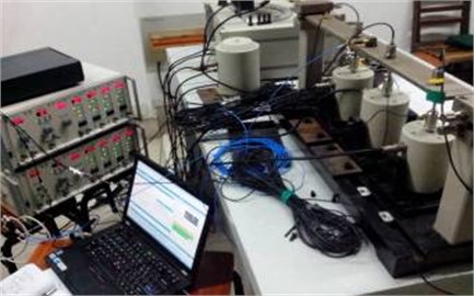
Table 1Separation effect of the first category excitation sources when using different blind separation methods
Model | Algorithm | s1 | s2 | s3 |
Transient | JADE | 0.8321 | 0.6542 | 0.2113 |
Improved JADE | 0.9201 | 0.8435 | 0.6544 | |
Convolution | Combined method | 0.9389 | 0.8945 | 0.8924 |
Table 2Separation effect of the second category excitation sources when using different blind separation methods
Model | Algorithm | s1 | s2 | s3 |
Transient | JADE | 0.7895 | 0.8253 | 0.3215 |
Improved JADE | 0.8957 | 0.7896 | 0.6589 | |
Convolution | Combined method | 0.9235 | 0.8654 | 0.8462 |
Table 1, Table 2 is separation effect comparison between the classical JADE algorithm, the improved JADE algorithm and the joint system method. The correlation coefficient of the joint system method is the largest in each source, and the coefficient of irrelevant source is relatively small. The separation effect of the joint method is more accurate and more practical.
7. Conclusions
A joint blind source separation algorithm for mechanical convolutional signal mixing is proposed, which is researched and experimentally applied. The conclusions are as follows:
The factors that influence the approximate diagonalization blind separation are studied, and the optimal approximation diagonalization blind separation based on the matrix distance as iterative parameters is proposed to improve the separation precision and stability of the transient mixed signal.
Developing the blind separation method of convolutional mixture, which is used as the separation algorithm of convolution hybrid model, and the mutual information between different sources in the whole frequency band is used to avoid the sorting problem between different frequencies of the same source. The system method of joint optimal approximate diagonalization can be applied to mechanical convoluted mixed signals.
The blind source separation algorithm proposed in this paper is based on independent component analysis, and its objective function reflects the independence of the source (non Gaussian maximum). When there are co frequency components or statistical correlation components, the zero time delay variance matrix of the source signal is not a diagonal matrix. Therefore, for the source signal with CO frequency, the algorithm is not applicable.
References
-
M. N. H. Mollah, S. Eguchi, and M. Minami, “Robust prewhitening for ICA by minimizing β-divergence and its application to FastICA,” Neural Processing Letters, Vol. 25, No. 2, pp. 91–110, Feb. 2007, https://doi.org/10.1007/s11063-006-9023-8
-
Z. Li, X. Yan, X. Wang, and Z. Peng, “Detection of gear cracks in a complex gearbox of wind turbines using supervised bounded component analysis of vibration signals collected from multi-channel sensors,” Journal of Sound and Vibration, Vol. 371, No. 9, pp. 406–433, Jun. 2016, https://doi.org/10.1016/j.jsv.2016.02.021
-
C. Rainieri, “Perspectives of second-order blind identification for operational modal analysis of civil structures,” Shock and Vibration, Vol. 2014, pp. 1–9, 2014, https://doi.org/10.1155/2014/845106
-
M. Toiviainen, F. Corona, J. Paaso, and P. Teppola, “Blind source separation in diffuse reflectance NIR spectroscopy using independent component analysis,” Journal of Chemometrics, Vol. 24, No. 7-8, pp. 514–522, Jul. 2010, https://doi.org/10.1002/cem.1316
-
J. Li, H. Zhang, and P. Wang, “Blind separation of temporally correlated noncircular sources using complex matrix joint diagonalization,” Pattern Recognition, Vol. 87, pp. 285–295, Mar. 2019, https://doi.org/10.1016/j.patcog.2018.10.016
-
H. Ghennioui, N. Thirion-Moreau, E. Moreau, and D. Aboutajdine, “Gradient-based joint block diagonalization algorithms: Application to blind separation of FIR convolutive mixtures,” Signal Processing, Vol. 90, No. 6, pp. 1836–1849, Jun. 2010, https://doi.org/10.1016/j.sigpro.2009.12.002
-
B. S. Kirei, M. D. Topa, I. Muresan, I. Homana, and N. Toma, “Blind source separation for convolutive mixtures with neural networks,” Advances in Electrical and Computer Engineering, Vol. 11, No. 1, pp. 63–68, 2011, https://doi.org/10.4316/aece.2011.01010
-
X. Zhang, X. P. Wu, Z. Lv, and X. J. Guo, “The improved method for solving permutation problem in frequency domain blind source separation of speech signals,” Advanced Materials Research, Vol. 433-440, pp. 7029–7034, Jan. 2012, https://doi.org/10.4028/www.scientific.net/amr.433-440.7029
-
S. M. Li and T. Yang., “Blind source separation based on kurtosis with applications to rotor vibration signal analysis,” (in Chinese), Chinese Journal of Applied Mechanics, Vol. 24, No. 4, pp. 560–566, 2007.
-
A. Ghazdali, M. El Rhabi, H. Fenniri, A. Hakim, and A. Keziou, “Blind noisy mixture separation for independent/dependent sources through a regularized criterion on copulas,” Signal Processing, Vol. 131, No. 2, pp. 502–513, Feb. 2017, https://doi.org/10.1016/j.sigpro.2016.09.006
-
Y. Y. Zhang, J. H. Xin, and Z. D. Zhao., “Study and application on joint diagonal blind identification with order cumulant,” (in Chinese), Journal of Huazhong University of Science and Technology (Natural Science Edition), Vol. 44, No. 7, pp. 86–90, 2016.
-
A. Brahmi, H. Ghennioui, C. Corbier, F. Guillet, and M. H. Lahbabi, “Blind separation of cyclostationary sources sharing common cyclic frequencies using joint diagonalization algorithm,” Mathematical Problems in Engineering, Vol. 2017, pp. 1–9, 2017, https://doi.org/10.1155/2017/2546838
-
J. Miao, G. Cheng, Y. Cai, and J. Xia, “Approximate joint singular value decomposition algorithm based on givens-like rotation,” IEEE Signal Processing Letters, Vol. 25, No. 5, pp. 620–624, May 2018, https://doi.org/10.1109/lsp.2018.2815584
-
A. Boudjellal, A. Mesloub, K. Abed-Meraim, and A. Belouchrani, “Separation of dependent autoregressive sources using joint matrix diagonalization,” IEEE Signal Processing Letters, Vol. 22, No. 8, pp. 1180–1183, Aug. 2015, https://doi.org/10.1109/lsp.2014.2380312
-
S. M. Li, H. D. Guo, and D. R. Li., “Review of vibration signal processing methods,” Chinese Journal of Scientific Instrument, Vol. 34, No. 8, pp. 1907–1915, 2013.
-
F. Bouchard, J. Malick, and M. Congedo, “Approximate joint diagonalization according to the natural Riemannian distance,” in Latent Variable Analysis and Signal Separation, Cham: Springer International Publishing, 2017, pp. 290–299, https://doi.org/10.1007/978-3-319-53547-0_28
-
M. E.-S. Waheed, M.-H. Mousa, and M.-K. Hussein, “Blind deconvolution of sources in Fourier space based on generalized laplace distribution,” International Journal of System Dynamics Applications, Vol. 2, No. 2, pp. 55–65, Apr. 2013, https://doi.org/10.4018/ijsda.2013040104
About this article

This work is supported by the National Nature Science Foundation of China (51405221), sponsored by Qing Lan Project and the Science and Technology Innovation Fund of Nanjing Institute of Technology (CKJB201408).
