Non-orthogonal joint block diagonalization based on the LU or QR factorizations for convolutive blind source separation

Zhang, Lei; Cao, Yueyun; Yang, Zichun; Weng, Lei

doi:10.21595/jve.2017.18039

Journal of Vibroengineering

Browse Journal

Submit article

Published: 15 August 2017

Check for updates

Non-orthogonal joint block diagonalization based on the LU or QR factorizations for convolutive blind source separation

Lei Zhang¹

Yueyun Cao²

Zichun Yang³

Lei Weng⁴

^{1, 2, 3, 4}Power Engineering college, Naval University of Engineering, WuHan 430033, P. R. China

Corresponding Author:

Lei Zhang

Cite the article Download PDF

Downloads 1351

WoS Core Citations 1

CrossRef Citations 1

Abstract

This article addresses the problem of blind source separation, in which the source signals are most often of the convolutive mixtures, and moreover, the source signals cannot satisfy independent identical distribution generally. One kind of prevailing and representative approaches for overcoming these difficulties is joint block diagonalization (JBD) method. To improve present JBD methods, we present a class of simple Jacobi-type JBD algorithms based on the LU or QR factorizations. Using Jacobi-type matrices we can replace high dimensional minimization problems with a sequence of simple one-dimensional problems. The novel methods are more general i.e. the orthogonal, positive definite or symmetric matrices and a preliminary whitening stage is no more compulsorily required, and further, the convergence is also guaranteed. The performance of the proposed algorithms, compared with the existing state-of-the-art JBD algorithms, is evaluated with computer simulations and vibration experimental. The results of numerical examples demonstrate that the robustness and effectiveness of the two novel algorithms provide a significant improvement i.e., yield less convergence time, higher precision of convergence, better success rate of block diagonalization. And the proposed algorithms are effective in separating the vibration signals of convolutive mixtures.

1. Introduction

Blind source separation (BSS) deals with the problem of finding both the unknown input sources and unknown mixing system from only observed output mixtures. BSS has recently become the focus of intensive research work due to its high potential in many applications such as antenna processing, speech processing and pattern recognition [1-3]. The recent successes of BSS might be also used in mechanical engineering [4-7]. In these reported applications for tackling the BSS, there were two kinds of BSS models i.e., instantaneous and convolutive mixture models. The instantaneous mixture models with a simple structure have been described in many papers and books [8-10]. However, when it came to deal with convolutive mixture signals, BSS might face a number of difficulties which seriously hindered its feasibility [11, 12]. There is currently an endeavor of research in separating convolutive mixture signals, yet no fully satisfying algorithms have been proposed so far.

Many approaches have been proposed to solve the convolutive BSS (CBSS) problem in recent years. One kind of prevailing and representative approaches is joint block diagonalization (JBD) which can produce potentially more elegant solution for CBSS in time domain [13]. In the article, we focus on the JBD problem, which has been firstly treated in [14] for a set of positive definite symmetric matrices. And then the same conditions also mentioned in [15]. To solve the JBD problem, Belouchrani have sketched several Jacobi strategies in [16-18]: the JBD problem was turn into a minimization problem which was processed by iterative methods; as a product of Givens rotations, each rotation made a block-diagonality criterion minimum around a fixed axis. Févotte and Theis [19, 20] have pointed out that the behavior of Jacobi approach was very much dependent on the initialization of the orthogonal basis and also on the choice of the successive rotations. Then they proposed some strategies to improve the efficiency of JBD. But there are also several critical constraints: the joint block-diagonalizer is an orthogonal (unitary in the complex case) matrix; the spatial pre-whitening is likely to lead to a larger error and, moreover, this error is unable to correct in the subsequent analysis. In [21] a gradient-based JBD algorithm have been used to achieve the same task but for non-unitary joint block-diagonalizers. This approach suffers from slow convergence rate since the iteration criteria possesses a fixed step size. To improve this shortcoming, some gradient-based JBD algorithms with optimal step size have been provided and studied in [22-24]. However, these algorithms are apt to converge to a local minimum and have low computational efficiency. To eliminate the degenerate solutions of the nonunitary JBD algorithm, Zhang [25] optimized a penalty term based weighted least-squares criterion. In [26], a novel tri-quadratic cost function was introduced, furthermore, an efficient algebraic method based on triple iterations has been used to search the minimum point of the cost function. Unfortunately, this method exists redundancy value and arises error when the mixture matrix is inversed. Some new Jacobi-like algorithms [27, 28] for non-orthogonal joint diagonalization have been proposed, but unfortunately cannot be used to solve the problem of block diagonalization.

Our purpose, here, is not only to tackle the problem of the approximate JBD by discard the orthogonal constraint on the joint block-diagonalizer i.e., impose as few assumptions as possible on the matrix set, but also to propose the JBD algorithms characterized by the merits of simplicity, effectiveness, and computational efficiency. Subsequently, we suggest two novels non-orthogonal JBD algorithms as well as the Jacobi-type schemes. The new methods are an extension of joint diagonalization (JD) algorithms [29] based on LU and QR decompositions mentioned in [30, 31] to the block diagonal case.

This article is organized as follows: the JBD problem is stated in Section 2.1. The two proposed algorithms are derived in section 2.2, whose convergence is proved in Section 2.3. In Section 3, we show how to apply the JBD algorithms to tackle the CBSS problem. Section 4 gives the results of numerical simulation by comparing the proposed algorithms with the state-of-the-art gradient-based algorithms introduced in [23]. In Section 5, the novel JBD algorithms are proved to be effective in separating vibration source of convolutive type, which outperforms JBD_OG and JRJBD algorithms [19].

2. Problem formulation and non-orthogonal JBD algorithms

2.1. The joint block diagonalization problem

Let ${\{R_{k}\}}_{k = 1}^{K} \in C^{M \times M}$ be a set of $K$ matrices (the matrices are square but not necessarily Hermitian or positive definite), that can be approximately diagonalized as:

1

R_{k} = A D_{k} A^{H} + N_{k},

where $A \in C^{M \times M}$ is a general mixing matrix and the matrix $N_{k} \in C^{M \times M}$ denotes residual noise, ${(\cdot)}^{H}$ denotes complex conjugate transpose (replace it by ${(\cdot)}^{T}$ in real domain). $D_{k} (k = 1, \cdot \cdot \cdot, K)$ is an $M \times M$ block diagonal matrix where the diagonal blocks are square matrices of any size and the off-diagonal blocks are zeros matrices i.e.:

2

D_{k} = [\begin{matrix} D_{k, 11} & \dots & 0_{1 r} \\ 0_{21} & \dots & 0_{2 r} \\ ⋮ & ⋱ & ⋮ \\ 0_{r 1} & \dots & D_{k, r r} \end{matrix}],

where $D_{k, i i}$ denotes the $i$ th diagonal block of the size $n_{i} \times n_{j}$ such that $n_{1} + n_{2} + \cdot \cdot \cdot + n_{r} = M$ . In general case, e.g. in the context of CBSS, the diagonal blocks are assumed to be the same size, i.e. $M = n_{i} \times r$ and where $0_{i j}$ denotes the $n_{i} \times n_{j}$ null matrix. The JBD problem consists of the estimation of $A$ and $D_{k} (k = 1, \cdot \cdot \cdot, K)$ when the matrices ${\{R_{k}\}}_{k = 1}^{K}$ are given. It can be noticed that the JBD model remains unchanged if one substitute $A$ by $A Λ P$ and $D_{k}$ by $P^{- 1} Λ^{- 1} D_{k} (P^{- 1} Λ^{- 1})^{H}$ , where $Λ$ is a nonsingular block diagonal matrix in which the arbitrary blocks are the same dimensions as $D_{k}$ . $P$ is an arbitrary block-wise permutation matrix. The JBD model is essentially unique when it is only subject to these indeterminacies of amplitude and permutation [24].

To this end, our aim is to present a new algorithm to solve the problem of the non-orthogonal JBD. The cost function with neglecting the noise term suggested in [23] is considered as follows:

3

C_{J B D} (B) = \sum_{k = 1}^{K} {‖O f f B d i a g (B R_{k} B^{H})‖}_{F}^{2} .

The above cost function can be regarded as the off-diagonal-block-error, our aim is to find a non-singular $B$ such that the $C_{J B D} (B)$ is as minimum as possible. Where ${‖\cdot‖}_{F}$ is the Frobenius norm and $B$ stands for inverse of the matrix $A$ (in BSS context, $B$ serves as the separating matrix). Considering the square matrix $R_{k} = (R_{k, i j}) \in C^{M \times M}$ :

R_{k} = [\begin{matrix} R_{k, 11} & \dots & R_{k, 1 r} \\ {R_{k,}}_{21} & \dots & {R_{k,}}_{2 r} \\ ⋮ & ⋱ & ⋮ \\ {R_{k,}}_{r 1} & \dots & R_{k, r r} \end{matrix}],

where $R_{k, i j}$ for all $i, j = 1, \cdot \cdot \cdot, r$ are $n_{i} \times n_{j}$ matrices (and $n_{1} + n_{2} + \cdot \cdot \cdot + n_{r} = M$ ) and two matrix operators $B d i a g (\cdot)$ and $O f f B d i a g (\cdot)$ can be respectively defined as:

B d i a g (R_{k}) = [\begin{matrix} R_{k, 11} & \dots & 0_{1 r} \\ 0_{21} & \dots & 0_{2 r} \\ ⋮ & ⋱ & ⋮ \\ 0_{r 1} & \dots & R_{k, r r} \end{matrix}], O f f B d i a g (R_{k}) = R_{k} - B d i a g (R_{k}) .

2.2. Two novel joint block diagonalization algorithms based LU and QR factorizations

Any non-singular matrix $B$ admits the LU factorization [30]:

4

B = P Λ L U,

where $L$ and $U$ are $M \times M$ unit lower and upper triangular matrices, respectively. A unit triangular matrix represents a triangular matrix with diagonal elements of one. $B$ also admits the QR factorization:

5

B = Λ Q U,

where $Q$ is $M \times M$ orthogonal matrix. Considering the JBD model’s indeterminacies, we note that any non-singular square separating matrix can be represented as these two types of decomposition. Here, we will implement the JBD in real domain (which is the problem usually encountered in BSS) i.e., in a real triangular and orthogonal basis. It is reasonable to consider the decompositions Eq. (4) or (5) and hence replace the minimization problem represented in Eq. (3) by two alternating stages involving the following sub-optimization:

6

\tilde{U} = a r g m i n \sum_{k = 1}^{K} {‖O f f B d i a g (U R_{k} U^{T})‖}_{F}^{2},

7a

\tilde{L} = a r g m i n \sum_{k = 1}^{K} {‖O f f B d i a g (L R_{k}^{'} L^{T})‖}_{F}^{2},

7b

\tilde{Q} = a r g m i n \sum_{k = 1}^{K} {‖O f f B d i a g (Q R_{k}^{'} Q^{T})‖}_{F}^{2},

where $R_{k}^{'} = \tilde{U} R_{k} {\tilde{U}}^{T}$ , $\tilde{L}$ , $\tilde{U}$ and $\tilde{Q}$ denote the estimates of $L$ , $U$ and $Q$ , respectively. Moreover, we adopt the Jacobi-type scheme to solve Eq. (6) and 7(a), 7(b) via a set of rotations.

The Jacobi matrix of lower unit triangular is denoted as $L_{i j} (a)$ , where the parameter $a$ corresponding to the position $(i, j)$ ( $i > j$ ) i.e., $L_{i j} (a)$ equals the identity matrix except the entry indexed $(i, j)$ is $a$ . In a similar fashion, we define the Jacobi matrix of unit upper triangular $U_{i j} (a)$ with parameter $a$ corresponding to the position $(i, j)$ ( $i > j$ ). In order to solve Eq. (6) and 7(a), we will firstly find the optimal $L_{i j} (a)$ and $U_{i j} (a)$ in each iteration. For fixed $a$ , one iteration of the method consists of

1. Solving Eq. (6) with respect to $a$ of $U_{i j} (a)$ , and.

Updating $R_{k} \leftarrow U_{i j} (a) R U_{i j} (a)^{T}$ for all $k$ (U-stage)

2. Solving Eq. (7a) with respect to $a$ of $L_{i j} (a)$ , and.

Updating $R_{k} \leftarrow L_{i j} (a) R L_{i j} (a)^{T}$ for all $k$ (L-stage)

We herein note that the proposed two non-orthogonal JBD algorithms are all of above-mentioned Jacobi-type, with the only differences on the adopted decompositions (LU or QR) and implementation details. Next, we give the details of the proposed algorithms. Following the Eq. (6), we have:

8

f (a) = a r g m i n {\sum_{k = 1}^{K} {‖O f f B d i a g (U_{i j} (a) R_{k} U_{i j} (a)^{T})‖}_{F}^{2}}_{}^{}

= a r g m i n a^{2} R_{1} + 2 a R_{2} + c o n s, i > L,

or = a r g m i n a^{2} R_{3} + 2 a R_{4} + c o n s, i \leq L,

where $L$ is the block dimension, $i, j = 1, \dots, M$ and $i < j$ .

R_{1} = \sum_{k = 1}^{K} {‖R_{k} ([L : i - 1, i + 1 : M], j)‖}_{F}^{2} + {‖R_{k} (j, [L : i - 1, i + 1 : M])‖}_{F}^{2},

\begin{array}{l} R_{2} = \sum_{k = 1}^{K} R_{k} (i, [L : i - 1, i + 1 : M]) R_{k} (j, [L : i - 1, i + 1 : M])^{T} \\ + \sum_{k = 1}^{K} R_{k} ([L : i - 1, i + 1 : M], i) R_{k} ([L : i - 1, i + 1 : M], j)^{T}, \end{array}

R_{3} = \sum_{k = 1}^{K} {‖R_{k} ([L + 1 : M], j)‖}_{F}^{2} + {‖R_{k} (j, [L + 1 : M])‖}_{F}^{2},

\begin{array}{l} R_{4} = \sum_{k = 1}^{K} R_{k} (i, [L + 1 : M]) R_{k} (j, [L + 1 : M])^{T} + \sum_{k = 1}^{K} R_{k} ([L + 1 : M], i) R_{k} ([L + 1 : M], j)^{T} . \end{array}

For matrix $R$ , $R (i, i n d e x)$ denotes a row-vector whose elements are from the $i$ th row of $R$ indexed by $i n d e x$ , the $A$ is a row vector $R (i n d e x, j)$ is defined similarly.

The computation of the optimal $\tilde{a}$ in Eq. (8) is:

9

\tilde{a} = - \frac{R_{2}}{R_{1}}, (i > L) or - \frac{R_{4}}{R_{3}}, (i \leq L) .

If $R_{1} = 0$ or $R_{3} = 0$ set $\tilde{a} = 0$ , i.e. $C_{J B D} (U)$ cannot be reduced by the particular $U_{i j} (a)$ .

As for the lower triangular matrices $L_{i j} (a)$ , we have similar result:

10

g (a) = a r g m i n \sum_{k = 1}^{K} {‖O f f B d i a g (L_{i j} (a) R_{k}^{'} L_{i j} (a)^{T})‖}_{F}^{2}

= a r g m i n a^{2} R_{1}^{'} + 2 a R_{2}^{'} + c o n s, i > L,

or = a r g m i n a^{2} R_{3}^{'} + 2 a R_{4}^{'} + c o n s, i \leq L,

where $L$ is the block dimension, $i, j = 1, \dots, M$ and $i > j$ :

i n d e x = [1 : i - 1, i + 1 : M],

i n d e x^{'} = i n d e x (L : M - 1), i \leq L,

i n d e x^{''} = i n d e x (l), i > L .

$l$ is a row vector in which element $l_{1}$ satisfy $⌈\frac{l_{1}}{L}⌉ \neq ⌈\frac{i}{L}⌉ l_{1} \in [1 : i - 1, i + : M]$ , $⌈X⌉$ rounds the elements of $X$ to the nearest integers towards infinity:

R_{1}^{'} = \sum_{k = 1}^{K} {‖R_{k}^{'} (i n d e x^{'}, j)‖}_{F}^{2} + {‖R_{k}^{'} (j, i n d e x^{'})‖}_{F}^{2},

R_{2}^{'} = \sum_{k = 1}^{K} R_{k}^{'} (j, i n d e x^{'}) R_{k}^{'} (i, i n d e x^{'})^{T} + R_{k}^{'} (i n d e x^{'}, j)^{T} R_{k}^{'} (i n d e x^{'}, i),

R_{3}^{'} = \sum_{k = 1}^{K} {‖R_{k}^{'} (i n d e x^{''}, j)‖}_{F}^{2} + {‖R_{k}^{'} (j, i n d e x^{''})‖}_{F}^{2},

R_{4}^{'} = \sum_{k = 1}^{K} R_{k}^{'} (j, i n d e x^{''}) R_{k}^{'} (i, i n d e x^{''})^{T} + R_{k}^{'} (i n d e x^{''}, j)^{T} R_{k}^{'} (i n d e x^{''}, i) .

The computation of the optimal $\tilde{a}$ value in Eq. (10):

11

\tilde{a} = - \frac{R_{2}^{'}}{R_{1}^{'}}, (i > L) or - \frac{R_{4}^{'}}{R_{3}^{'}}, (i \leq L) .

If $R_{1}^{'} = 0$ or $R_{3}^{'} = 0$ set $\tilde{a} = 0$ , i.e. $C_{J B D} (L)$ cannot be reduced by the particular $L_{i j} (a)$ . The computation of the optimal parameter $\tilde{a}$ requires solving a polynomial of degree 2 in the real domain, which is more effective than other JBD methods that need to solve a polynomial of degree 4, such as JBD_OG, JBD_ORG and JBD-NCG,etc. [22-24].

In the QR algorithm, we consider the QR decomposition of $Β$ , hence the sub-optimization problem in the Q-stage in Eq. 7(b) is indeed an orthogonal JBD problems which can be solved by Févotte’s Jacobi-type algorithm [19]. Févotte indicated that the behavior of the Jacobi approach was very much dependent on the initialization of the orthogonal basis, and also relied on the choice of the successive rotations. Here, the algorithm is initialized with the matrix $Q_{J D}$ provided by joint diagonalization of $R_{k}$ , and consists of choosing at each iteration the couple $(p, q)$ ensuring a maximum decrease of criterion $C_{J B D} (Q)$ .

Now that we have obtained the U-stage and L-stage (Q-stage) for the proposed algorithm, we loop these two stages until convergence is reached. In addition, we note that there would be several ways to control the convergence of the JBD algorithms. For example, we could stop the iterations when the parameter values in each iteration of the U-stage or L-stage (Q-stage) are small enough, which indicates a minute contribution from the elementary rotations, and hence convergence. We may as well monitor the sum off-diagonal squared norms $C_{J B D} (B)$ in iteration, and stop the loops when the change in it is smaller than a preset threshold. The values of ${‖L U - I‖}_{F}^{2} < ε$ between two successive complete runs of U-stage and L-stage are usually used as a terminate criteria. Here, we stop the iteration when the values $I_{o f f} = \sum_{k = 1}^{K} {‖O f f B d i a g (R_{k})‖}_{F}^{2} / \sum_{k = 1}^{K} {‖B d i a g (R_{k})‖}_{F}^{2} < ε$ , which can reflect relative change between off-block diagonal and block diagonal. And this criterion can be adapted to all of iterative methods for solving JBD problem, which can also give a more intuitive comparison between these methods. Therefore, this terminate criteria is much more rational and effective. In the following context of our manuscript, we will use one of the following terminate criteria

(st1) $I_{o f f} < 1 0^{- 7}$ ;

(st2) $|C_{J B D}^{t + 1} - C_{J B D}^{t}| / C_{J B D}^{t} < 1 0^{- 7}$ ;

(st3) $|I_{c o n v}^{t + 1} - I_{c o n v}^{t}| < 1 0^{- 5}$ (mentioned at section 4).

We name the novel JBD approaches based on LU and QR factorizations as LUJBD and QUJBD, respectively, and summarize them as following:

1. Set $B = I$ .

2. U-stage (R-stage): set $U = I$ , for $1 \leq i < j \leq M$

Find ${\tilde{a}}_{i j} = a r g m i n_{a} C_{J B D} (U_{i j} (a))$ from Eq. (9)

Update $R_{k} \leftarrow U_{i j} ({\tilde{a}}_{i j}) R_{k} U_{i j} ({\tilde{a}}_{i j})^{T}$ and $U \leftarrow U_{i j} ({\tilde{a}}_{i j}) U$

3. L-stage (Q-stage): set $L = I$ ( $Q = Q_{J D}$ ), for $1 \leq j < i \leq M$

Find ${\tilde{a}}_{i j} = a r g m i n_{a} C_{J B D} (L_{i j} (a))$ from Eq. (11) ( $θ_{i j} = a r g m i n_{θ} C_{J B D} (U_{i j} (θ))$ from [20])

Update $R_{k} \leftarrow L_{i j} ({\tilde{a}}_{i j}) R_{k} L_{i j} ({\tilde{a}}_{i j})^{T}$ ( $R_{k} \leftarrow G_{i j} (θ_{i j}) R_{k} G_{i j} (θ_{i j})^{T}$ )

and $L \leftarrow L_{i j} ({\tilde{a}}_{i j}) L$ ( $Q \leftarrow G_{i j} (θ_{i j}) Q$ )

4. If the terminate criteria from (st1), (st2) or (st3) isn’t satisfied completely, then $B \leftarrow L U B$ ( $B \leftarrow Q U B$ ) and go to 2, else end.

We replace each of these $M (M - 1) / 2$ dimensional minimization problems by a sequence of simple one-dimensional problems via using triangular and orthogonal Jacobi matrices. Note that for updating $R_{k}$ , the matrix multiplications can be realized by few vectors scaling and vector. In additions, this will cost fewer time than other method of non-orthogonal JBD [22-24]. And the existence and uniqueness of joint block diagonalization of this cost function has been proved in [20].

2.3. Convergence of the algorithm

By construction, the algorithm ensures decrease of criterion $C_{J B D} (B)$ at iteration process. According to Eq. (8) or (10), we have:

C_{J B D} (U^{t + 1}) - C_{J B D} (U^{t}) = {\tilde{a}}^{2} R_{c} + 2 \tilde{a} R_{d} .

Respectively $R_{c} = R_{1}, R_{3}, R_{1}^{'}$ , $R_{3}^{'}$ , $R_{d} = R_{2}, R_{4}, R_{2}^{'}, R_{4}^{'}$ and $R_{c} > 0$ .

Replace $\tilde{a}$ from Eqs. (9) or (11):

12

C_{J B D} (U^{t + 1}) - C_{J B D} (U^{t}) = {\tilde{a}}^{2} R_{c} + 2 \tilde{a} R_{d} = - \frac{R_{d}^{2}}{R_{c}} \leq 0 .

Only $R_{c} = 0$ or $R_{d} = 0$ set $\tilde{a} = 0$ , Eq. (12) is putted equal sign, but usually $R_{c} \neq 0$ and $R_{d} \neq 0$ in CBSS mentioned in Section 3.

Similarly, $C_{J B D} (L^{t + 1}) - C_{J B D} (L^{t}) \leq 0,$ or $C_{J B D} (Q^{t + 1}) - C_{J B D} (Q^{t}) \leq 0$ has been proved in [20].

At each iteration of the algorithm, the matrix $R_{k}^{t + 1}$ obtained after rotations is thus ‘at least as diagonal as’ matrix $R_{k}^{t}$ at previous iteration. Since every bounded monotonic sequence in real matrix domain, the convergence of our algorithm is guaranteed.

3. Application to CBSS

The problems of convolutive BSS (CBSS) occur in various applications. One typical application is in blind separation of vibration signals, which is fully studied in this paper for detecting the solution of the CBSS problems. The CBSS consists of estimating a set of unobserved source signals from their convolutive mixtures without requiring a priori knowledge of the sources and corresponding mixing system. Then the CBSS can be identified by means of JBD of a set of covariance matrices. We consider the following discrete-time MIMO model [25]:

13

X (t) = \sum_{l^{'} = 0}^{L^{'}} H (l^{'}) S (t - l^{'}) + N (t),

where $t$ is the discrete time index, $l^{'} = 1, \dots, L^{'},$ $L^{'}$ denotes FIR filter’s length. $S (t) = {[s_{1} (t), \cdot \cdot \cdot, s_{m} (t)]}^{T}$ denotes source signal vector with the source numbers are $m$ , and $X (t) = {[x_{1} (t), \cdot \cdot \cdot, x_{n} (t)]}^{T}$ is the mixing signal vector obtained by $n$ observation signals. In the mixing linear time-invariant system, the matrix-type impulse response $H (l^{'}) = [h_{1} (l^{'}), \cdot \cdot \cdot, h_{m} (l^{'})]$ consists of channel impulse responses $h_{i j} (l^{'})$ $(i = 1, \dots, n,$ $j = 1, \dots, m)$ . Aiming to the received signal on the $i$ th array element, we take the $P + 1$ sliding window and constitute a column vector:

x_{i} (t) = [x_{i} (t), x_{i} (t - 1), \cdot \cdot \cdot, x_{i} (t - P)]^{T}, i = 1,2, \dots, n .

Then putting the array element processed by sliding window together and defining the observed signal vector:

\bar{X} (t) = [x_{1} (t), x_{2} (t), \cdot \cdot \cdot, x_{n} (t)]^{T} .

Hence:

14

\bar{X} (t) = H \bar{S} (t) + N (t),

where $\bar{S} (t) = [s_{1} (t), s_{2} (t), \cdot \cdot \cdot, s_{m} (t)]^{T}$ , and:

s_{j} (t) = [s_{j} (t), s_{j} (t - 1), \cdot \cdot \cdot, s_{j} (t - L^{'} - P + 1)]^{T},

H = [\begin{matrix} H_{11} & \dots & H_{1 m} \\ H_{21} & \dots & H_{2 m} \\ ⋮ & ⋱ & ⋮ \\ H_{n 1} & \dots & H_{n m} \end{matrix}]

$H_{i j}$ is block element of $H$ which matrix dimension is $(P + 1) \times (L^{'} + P)$ , and:

H_{i j} = [\begin{matrix} h_{i j} (0) & h_{i j} (1) & \dots & h_{i j} (L^{'} - 1) & 0 & \dots & 0 \\ 0 & h_{i j} (0) & \dots & h_{i j} (L^{'} - 2) & h_{i j} (L^{'} - 1) & \dots & 0 \\ ⋮ & ⋱ & ⋮ & ⋱ & ⋱ & ⋱ & ⋮ \\ 0 & \dots & 0 & h_{i j} (0) & \dots & h_{i j} (L^{'} - 2) & h_{i j} (L^{'} - 1) \end{matrix}] .

The following assumptions concerning the above mixture model Eq. (14) have to be made to ensure that it is possible to apply the proposed algorithms to CBSS [25].

Assumption 1. The source signals are zero mean, individually correlated in time but mutually uncorrelated, i.e., for all time delay $τ$ , the cross correlation functions $r_{s_{i} s_{j}} (t, τ) = 0$ , $\forall i \neq j$ , and the auto-correlation functions $r_{s_{i} s_{i}} (t, τ) \neq 0$ , $i = 1, \dots, m$ . Meanwhile, the source signals have a different auto-correlation function.

Assumption 2. The sensor noises $N (t)$ are zero mean, independent identically distributed with the same power $σ_{N}^{2}$ . The noises are assumed to be independent with the sources.

Assumption 3. The mixing matrix $H$ is assumed as column full rank. This requires that the length of the sliding window $P$ satisfies $n (P + 1) \geq m (P + L^{'})$ .

Assumption 1 is the core assumption. As is shown in [25], this assumption enables us to separate the sources from their convolutive mixtures by diagonalizing the second-order statistic of the reformulated observed signals (this will be addressed below). Assumption 2 enables us to easily deal with the noise and Assumption 3 guarantees that the mixing system is invertible, therefore it is a necessary condition that the source signals can be completely separated.

Under these assumptions, the spatial covariance matrices of the observations satisfy:

15

R_{\bar{x}} (t, t - τ_{k}) = E (\bar{x} (t) {\bar{x}}^{T} (t - τ_{k})) = H R_{\bar{s}} (t, t - τ_{k}) H^{T} + R_{N} (t, t - τ_{k}),

where $τ_{k} \in [0,1, 2, \dots, q - 1] (k = 1, \dots, K)$ is the successive time delays, $R_{N} (t, t - τ_{k})$ is computed according to [26]. It can be deduced from the above assumptions that in Eq. (15) the matrices take the following forms, respectively:

R_{\bar{x}} (τ_{k}) = [\begin{matrix} R_{x_{1} x_{1}} (τ_{k}) R_{x_{1} x_{2}} (τ_{k}) & \dots & R_{x_{1} x_{n}} (τ_{k}) \\ R_{x_{2} x_{1}} (τ_{k}) R_{x_{2} x_{2}} (τ_{k}) & \dots & R_{x_{2} x_{n}} (τ_{k}) \\ ⋮ & ⋱ & ⋮ \\ R_{x_{n} x_{1}} (τ_{k}) R_{x_{n} x_{2}} (τ_{k}) & \dots & R_{x_{n} x_{n}} (τ_{k}) \end{matrix}] \in R^{(P + 1) n \times (P + 1) n},

R_{\bar{s}} (τ_{k}) = [\begin{matrix} R_{s_{1} s_{1}} (τ_{k}) & 0 & \dots & 0 \\ 0 & R_{s_{2} s_{2}} (τ_{k}) & \dots & 0 \\ ⋮ & ⋮ & ⋱ & ⋮ \\ 0 & 0 & \dots & R_{s_{m} s_{m}} (τ_{k}) \end{matrix}] \in R^{(P + L^{'}) m \times (P + L^{'}) m},

where the block matrices in $R_{\bar{x}} (τ_{k})$ and $R_{\bar{s}} (τ_{k})$ have the following form:

R_{x_{i} x_{j}} (τ_{k}) = E (x_{i} (t) x_{j}^{T} (t - τ_{k}))

[\begin{matrix} r (0, - τ_{k}) & r (0, - τ_{k} - 1) & \dots & r (0, - τ_{k} - P) \\ r (- 1, - τ_{k}) & r (- 1, - τ_{k} - 1) & \dots & r (- 1, - τ_{k} - P) \\ ⋮ & ⋮ & ⋱ & ⋮ \\ r (- P, - τ_{k}) & r (- P, - τ_{k} - 1) & \dots & r (- P, - τ_{k} - P) \end{matrix}] \in R^{(P + 1) \times (P + 1)},

where $r (- a, - b) = E (x_{i} (t - a) x_{j}^{T} (t - b))$ , $R_{s_{i} s_{i}} (τ_{k})$ have the similar form, which is the $(L^{'} + P) \times (L^{'} + P)$ matrix. According to the Eq. (15), a group of matrices $R = \{R_{k}, k = 1, \dots, K\}$ which can be block diagonalized, and satisfy $R_{k} = A D_{k} A^{T}$ , $D_{k}$ have diagonalization structure. Hence, The JBD method mentioned in section 2.2 can be used to solve CBSS problem. Once the joint block diagonalizer $B$ is determined, the recovered signals are obtained up to permutation and a filter by:

16

\hat{S} (t) = B \bar{X} (t) .

It is worth mentioning that the indeterminacies of amplitude and permutation exist in JBD algorithms correspond to the well-known indeterminacies in CBSS. The correlation matrices $R_{\bar{x}} (τ_{k})$ is actually replaced by their discrete time series estimate. To acquire a good estimate of the discrete correlation matrices, we may divide the observed sequences (the output of the reformulated model (15)) into the appropriate length of the sample.

4. Numerical simulations

Simulations are now provided to illustrate the behavior and the performance of the proposed JBD algorithms (LUJBD, QRJBD). We will also compare the proposed algorithms with the JBD_OG, JBD_ORG in the robustness and efficiency by generating random dates. To achieve these purposes, a set of real block-diagonal matrices $D_{k}$ (for all $k = 1, \dots, K$ ) are devised from random entries with a Gaussian distribution of zero mean and unit variance. Then, random noise entries with a Gaussian distribution of zero mean and variance $σ_{N}^{2}$ will be added on the off-diagonal blocks of the previous matrices $D_{k}$ . A signal to noise ratio can be defined as $S N R = 10 l o g (1 / σ_{N}^{2})$ .

To measure the quality of the different algorithms, the following performance index is used [22]:

I_{c o n v} (G) = \frac{1}{r (r - 1)} [\sum_{i = 1}^{r} (\sum_{j = 1}^{r} \frac{{‖G_{i j}‖}_{F}^{2}}{m a x_{l} {‖G_{i l}‖}_{F}^{2}} - 1) + \sum_{j = 1}^{r} (\sum_{i = 1}^{r} \frac{{‖G_{i j}‖}_{F}^{2}}{m a x_{l} {‖G_{l j}‖}_{F}^{2}} - 1)],

where $G_{i j}$ ( $i, j \in \{1, \cdot \cdot \cdot, r\}$ ) denotes the $(i, j)$ th block matrix of $G = \tilde{B} A$ . This index will be used in the CBSS, which can take into account the inherent indetermination of the BSS problem. It is clearly that the smaller the index performance $I_{c o n v} (G)$ , the better the separation quality. Regarding to the charts, $I_{c o n v} (G)$ is often given in dB i.e., $I_{c o n v} (G) d B = 10 l o g (I_{c o n v} (G))$ . In all the simulations, the true mixing matrix $A$ or $H$ has been randomly chosen with zero mean and unit variance.

In Fig. 1 and Fig. 2, we focus on the exactly determined case $M =$ 9, $L =$ 3, $K =$ 20, $S N R =$ 60 dB, the results have been averaged over 100 runs. Fig. 1 represents the percentage of successful runs, where a run is declared successful w.r.t. the following criteria satisfy: $I_{c o n v} < 1 0^{- 7}$ , (st1), (st2). Fig. 2 represents the average running time per successful convergence. Comparing the LUJBD and QRJBD approaches with the state-of-the-art JBD_OG, and JBD_ORG., we can confirm that the approaches proposed in Section 2.2 improve the performance of JBD better than the gradient-based methods: the LUJBD and QRJBD methods converge to the global minimum more frequently, see Fig. 1, and faster see Fig. 2 than JBD_OG, JBD_ORG. Under the same terminated criteria, it can be observed that the LUJBD and QRJBD methods also outperform the JBD_OG, JBD_ORG methods, and the LUJBD method show the best performance. We can also conclude that the sensitivity of the different convergence termination criteria for different JBD methods is diverse and, moreover, the percentage of successful runs and average running time are also varying. In other words, we should choose appropriate terminate criteria which is able to obtain the accuracy of block diagonalization, goodness of success rate and convergence speed.

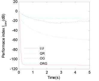
In Fig. 3 we focus on the exactly determined case $M =$ 9, $L =$ 3, $K =$ 20, $S N R =$ 60 dB, the results have been averaged over 100 runs. Because various approaches have different iteration time of each step, Here, we consider all methods converge to the same time, which is more reasonable than converge to certain iteration steps mentioned in [23, 25]. The evolution of the performance index versus the convergence time shows that the convergence performance of the LUJBD and QRJBD methods is better than the JBDOG and JBDORG method. The LUJBD and QRJBD algorithms cost less time when performance index $I_{c o n v}$ reaches a stable convergence level, and have smaller value of performance index $I_{c o n v}$ when all algorithms converge to same time. In other words, the BSS methods proposed in this paper possess less convergence time, higher precision of convergence, faster convergence speed.

Fig. 1The percentage of successful runs

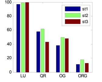
Fig. 2The average running time per successful convergence

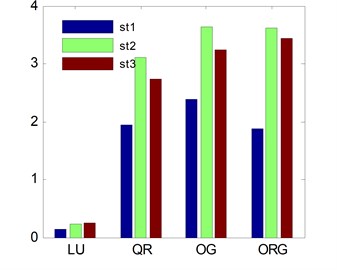
Fig. 3Average performance index Iconv versus the convergence time for LUJBD, QLJBD, JBDOG, JBDORG algorithms. SNR=60 and K= 20 matrices

In Fig. 4, we discuss the number of the matrices how to affect the performance. The results have been averaged over 100 runs. We devise the same stop criteria i.e., one of the terminate criteria (st1), (st2) and (st3) is satisfied. We set $M =$ 9, $L =$ 3, $S N R =$ 60 dB. The following observations can be made: the more matrices to be joint block-diagonalized, the better performance we can obtain. But the computational cost also increases when the number of matrix rises. Therefore, the choice of matrix number should combine the accuracy of JBD algorithms with complexity of JBD algorithms. From Fig. 4, the matrix number 20 is a better choice. The LUJBD algorithm with better convergence turned out to be slightly superior to other JBD algorithms.

Fig. 4Average Iconv versus the number of matrices for LUJBD, QLJBD, JBDOG, JBDORG algorithms. SNR= 60 and avarage 100 runs

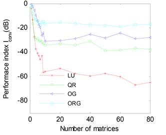
Fig. 5Average Iconv versus SNR for LUJBD, QLJBD, JBDOG, JBDORG algorithms. K= 20 and avarage 100 runs

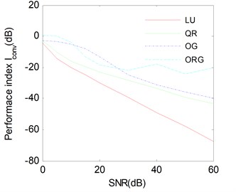
With the same stop criteria and other assumptions in Fig. 4, one can observe from Fig. 5 that when the SNR grows, the average performance of each algorithm becomes better except few fluctuation points. The noise sensitivity of LUJBD is slightly higher that the remaining three kinds of methods, however, for a given value of SNR, the average performance index of LUJBD and QLJBD is always better than that of two gradient-based methods.

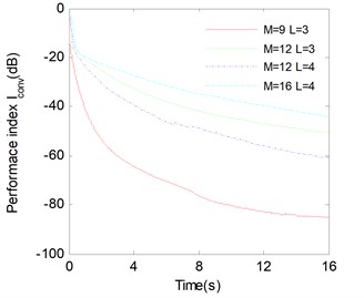
Finally, in Fig. 6 and Fig. 7, we study separation performance versus matrix dimension $M$ and the block dimension $L$ for both algorithms ( $K =$ 20, $S N R =$ 60 dB), the results have been averaged over 100 runs. One can observe that in the same block dimension $L$ case, the larger the matrix dimension $M$ , the weaker the estimation accuracy of mixing matrix. And in the same matrix dimension $M$ case, the larger the block dimension $L$ , the better the estimation accuracy of mixing matrix. Therefore, we can improve the performance index by increasing the number of the matrix $K$ and the block dimension $L$ when the dimension of target matrix increases.

Fig. 6Average Iconv versus the convergence time with different M and L for LUJBD algorithms. SNR=60 and K= 20 matrices

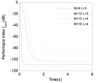
Fig. 7Average Iconv versus the convergence time with different M and L for QLJBD algorithms. SNR=60 and K= 20 matrices

5. Applying CBSS to the vibration source separation

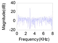
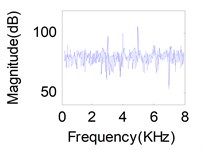
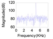
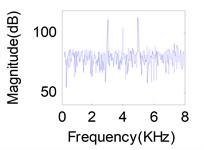
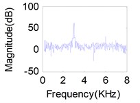
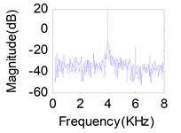
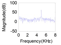
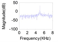
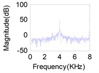
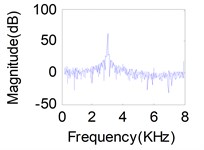
The experimental model is a double-stiffened cylindrical shell depicted in Fig. 8, which is used to simulate the cabin model. Underwater vibration tests of the double-stiffened cylindrical shell were carried out in anechoic water pool with a length of 16 meters, a width of 8 meters and a height of 8 meters. In the double-stiffened cylindrical shell, three exciters were arranged in the front part (No. 1 excitation source), middle part (No. 2 excitation source), rear part (No. 3 excitation source), respectively, which were used to simulate vibration sources of the internal equipment. Twenty-nine vibration acceleration sensors were arranged in the inner shell, and four accelerometers containing abundant vibration information were arranged in the vicinity of each excitation point. The location of exciters and acceleration sensors were shown in Fig. 9. Only the vertical excitation and response were considered in this test, and the model was located underwater 3.75 m. During the test, three exciters were controlled on the shore, and each exciter was turned on separately or multiple exciters were operated simultaneously according to different test requirements. Three exciters launched a continuous sinusoidal signal with different excitation frequencies and same energy, the frequency was 5 kHz, 4 kHz, 3 kHz, corresponding to No. 1 exciter, No. 2 exciter and No. 3 exciter. The vibration data was collected when the exciter was in stable operation. The sampling frequency was 16384 Hz and the sampling time was 10 s.

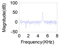
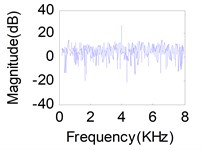
Fig. 11(d), (e), (f) show the mixture signals obtained by three sensors (17, 20, 23) on the inner shell when all of the exciters act simultaneously. It is obvious that the mix-signals with mutual spectrum aliasing are not able to represent real vibration characteristics and be utilized directly. We can also demonstrate that a mixture of vibrations is most often of the convolutive type which is not prone to be tackled, and moreover, the independence among the vibration sources is often not satisfactory strictly. Therefore, it is difficult to separate mechanical vibration source using traditional source separation methods. However, we propose the Jacobi-type JBD algorithms based on the LU or QR factorizations in this article, which can overcome above shortcomings effectively.

To ensure the stability of the solution, the terminate criteria $ε = a b s (I_{o f f}^{t + t_{1}} - I_{o f f}^{t + t_{1} + 1}) < 1 0^{- 6}$ $(t_{1} = 0, \dots, 9)$ is selected. We select observed signals $n =$ 5 i.e., sensors 17, 20, 23, 26, 29，and source signals $m =$ 3. The model parameters including $L^{'}$ , $P$ , $K$ are selected to guarantee that the solution accuracy satisfy $I_{o f f} \leq$ –35 dB. The filter length $L^{'} =$ 13, the sliding window $P =$ 17 and a set of covariance matrices $K =$ 30 with a time lag $τ_{k}$ taking linearly spaced valued.

In Fig. 10, the evolution of the performance index $I_{o f f}$ versus the convergence time shows that the convergence performance of the LUJBD and QRJBD methods are superior to the JBDOG and JRJBD methods [20]. The LUJBD and QRJBD algorithms cost less time when $I_{o f f} <$ –20 dB, and have smaller performance index $I_{o f f}$ when the convergence time is same. In other words, the BSS methods proposed in this paper possess higher precision of convergence, faster convergence speed. The low computational accuracy and efficiency of the latter two algorithms are mainly due to following reasons: (1) the JBDOG algorithm generally suffers from slow convergence rate and is apt to converge to a local minimum; and the accuracy of blind source separation is often hindered by the inversion of ill-conditioned matrices. (2) the joint block-diagonalizer of JRJBD algorithm is an orthogonal matrix, the spatial pre-whitening which is likely to lead to a larger error need to be applied. Moreover, this error is unable to correct in the subsequent analysis.

Fig. 11(a), (b), (c) represents source signals acquired by the acceleration sensors near excitation point (Here, we choose acceleration sensors 1, 8, 14 which have a higher signal-to-noise ratio) when each of the exciter act respectively. Comparison between the recovered primary sources – see Fig. 11(g), (h), (i) for LUJBD model and (j), (k), (l) for QRJBD model – with the true one shows that the proposed separation algorithms only subjected to indeterminacies of the permutation and amplitude are effective.

Fig. 8The experimental cabin model

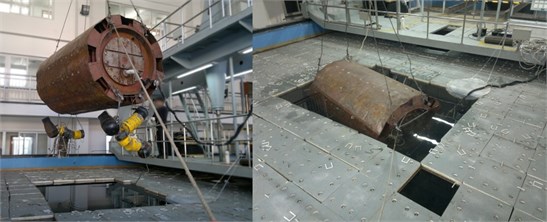
Fig. 9The location of exciters and acceleration sensors

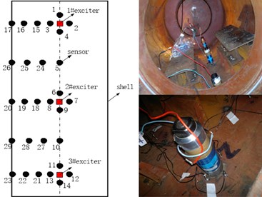
Fig. 10Average performance index Iconv versus the convergence time for four algorithms. K= 30, L'= 13, P= 17

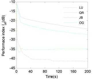
Fig. 11Separation results for known channel-Sources: a) s1, b) s2, c) s3. Mixtures: d) x1, e) x2, f) x3. Separation sources for LUJBD: g) s1', h) s2', i) s3'. Separation sources for QLJBD: j) s1'', k) s2'', l) s3''

Separation results for known channel-Sources: a) s1, b) s2, c) s3. Mixtures: d) x1, e) x2, f) x3. Separation sources for LUJBD: g) s1', h) s2', i) s3'. Separation sources for QLJBD: j) s1'', k) s2'', l) s3''

a)

b)

c)

d)

e)

f)

g)

h)

i)

j)

k)

l)

6. Conclusions

In this article, to solve the convolutive BSS (CBSS) problem, we present a class of simple Jacobi-type JBD algorithms based on the LU or QR factorizations. Using Jacobi-type matrices we can replace high dimensional minimization problems with a sequence of simple one-dimensional problems. The two novel methods named LUJBD and QRJBD are no more necessarily orthogonal, positive definite or symmetric matrices. In addition, we propose a novel convergence criteria which can reflect relative change between off-block diagonal and block diagonal. And this criterion can be adapted to all of iterative methods for solving JBD problem, which can also give a more intuitive comparison between different methods. The computation of the optimal parameter requires solving a polynomial of degree 2 in the real domain in LUJBD and QRJBD methods, which is more effective than other JBD methods that need to solve polynomial of degree 4. Therefore, the two new algorithms will cost fewer times than other non-orthogonal JBD methods, and moreover, the convergence of these two algorithms is also guaranteed.

A series of comparisons of the proposed approaches with the state-of-the-art JBD approaches (JBD_OG and JBD_ORG) based on gradient algorithms are implemented by varieties of numerical simulations. The results show that the LUJBD and QRJBD methods converge to the global minimum more frequently, and faster than JBD_OG, JBD_ORG. Choosing appropriate terminate criteria is beneficial to obtain the accuracy of block diagonalization, goodness of success rate and convergence speed. It can be readily observed that the more target matrices selected to be joint block-diagonalized, the better performance we can obtain. But the computational cost also increases when the number of matrix rises. Therefore, the choice of matrix number should combine algorithm accuracy with complexity. We can also improve the performance index by increasing the block dimension and decreasing the matrix dimension. Then the two novel JBD algorithms and the JBD_OG, JRJBD methods for separating practical vibration sources are studied. We can conclude that the convergence performance and accuracy of the LUJBD and QRJBD methods are superior to the JBD_OG and JRJBD methods. Finally, Comparison the recovered primary sources with the true one demonstrates the validity of the proposed algorithms for separating the vibration signals of convolutive mixtures.

References

Castell M., Bianchi P., Chevreuil A., et al. A blind source separation framework for detecting CPM sources mixed by a convolutive MIMO filter. Signal Processing, Vol. 86, 2006, p. 1950-1967.

Publisher
Zhang Y., Zhao Y. X. Modulation domain blind speech separation in noisy environments. Speech Communication, Vol. 55, Issue 10, 2013, p. 1081-1099.

Publisher
Pelegrina G. D., Duarte L. T., Jutten C. Blind source separation and feature extraction in concurrent control charts pattern recognition: novel analyses and a comparison of different methods. Computers and Industrial Engineering, Vol. 92, 2016, p. 105-114.

Publisher
Popescu T. D. Blind separation of vibration signals and source change Detection: Application to machine monitoring. Applied Mathematical Modelling, Vol. 34, 2010, p. 3408-3421.

Publisher
McNeill S. I., Zimmerman D. C. Relating independent components to free-vibration modal responses. Shock and Vibration, Vol. 17, 2010, p. 161-170.

Publisher
Lee D. S., Cho D. S., Kim K., et al. A simple iterative independent component analysis algorithm for vibration source signal identification of complex structures. International Journal of Naval Architecture and Ocean Engineering, Vol. 7, Issue 1, 2015, p. 128-141.

Publisher
Li Y. B., Xu M. Q., Wei Y., et al. An improvement EMD method based on the optimized rational Hermite interpolation approach and its application to gear fault diagnosis. Measurement, Vol. 63, 2015, p. 330-345.

Publisher
Popescu T. D. Analysis of traffic-induced vibrations by blind source separation with application in building monitoring. Mathematics and Computers in Simulation, Vol. 80, 2010, p. 2374-2385.

Publisher
Babaie-Zadeh M., Jutten C. A general approach for mutual information minimization and its application to blind source separation. Signal Processing, Vol. 85, 2005, p. 975-995.

Publisher
Jing J. P., Meng G. A novel method for multi-fault diagnosis of rotor system. Mechanism and Machine Theory, Vol. 44, 2009, p. 697-709.

Publisher
Antoni J. Blind separation of vibration components: principles and demonstrations. Mechanical Systems and Signal Processing, Vol. 19, 2005, p. 1166-1180.

Publisher
Rhabi M. E., Fenniri H., Keziou A., et al. A robust algorithm for convolutive blind source separation in presence of noise. Signal Processing, Vol. 93, 2013, p. 818-827.

Publisher
Bousbia-Salah H., Belouchrani A., Abed-Meraim K. Blind separation of convolutive mixtures using joint block diagonalization. International Symposium on Signal and its Applications(ISSPA), Kuala Lumpur, Malaysia, 2001, p. 13-16.

Publisher
Flury B. D., Neuenschwander B. E. Simultaneous diagonalization algorithm with applications in multivariate statistics. International Series of Numerical Mathematics, Vol. 19, 1994, p. 179-205.

Publisher
Pham D. T. Blind separation of cyclostationary sources using joint block approximate diagonalization. Lecture Notes in Computer Science, Vol. 4666, 2007, p. 244-251.

Publisher
Belouchrani A., Amin M. G., Abed-Meraim K. Direction finding in correlated noise fields based on joint block-diagonalization of spatio-temporal correlation matrices. IEEE-SP Letters, 1997, p. 266-268.

Publisher
Belouchrani A., Abed-Meraim K., Hua Y. Jacobi like algorithms for joint block diagonalization: Application to source localization. Proceedings of IEEE International Workshop on Intelligent Signal Processing and Communication Systems, Melbourne, 1998.

Search CrossRef
Abed-Meraim K., Belouchrani A. Algorithms for joint block diagonalization. 12th European Signal Processing Conference, Vienna, Austria, 2004, p. 209-212.

Search CrossRef
Févotte C., Theis F. J. Pivot selection strategies in Jacobi joint block-diagonalization. Lecture Notes in Computer Science, Vol. 4666, 2007, p. 177-184.

Publisher
Févotte C., Theis F. J. Orthonormal Approximate Joint Block-Diagonalization. Technical Report GET/Telecom Paris 2007D007, 2007, p. 1-24.

Search CrossRef
Ghennioui H., Fadaili E. M., Thirion Moreau N., et al. A non-unitary joint block diagonalization algorithm for blind separation of convolutive mixtures of sources. IEEE Signal Processing Letters, Vol. 14, Issue 11, 2007, p. 860-863.

Publisher
Ghennioui H., Thirion Moreau N., Moreau E., et al. Non-unitary joint-block diagonalization of complex matrices using a gradient approach. Lecture Notes in Computer Science, Vol. 4666, 2007, p. 201-208.

Publisher
Ghennioui H., Thirion-Moreau N., Moreau E., et al. Gradient-based joint block diagonalization algorithms: application to blind separation of FIR convolutive mixture. Signal Processing, Vol. 90, 2010, p. 1836-1849.

Publisher
Nion D. A tensor framework for nonunitary joint block diagonalization. IEEE Transactions on Signal Processing, Vol. 59, Issue 10, 2011, p. 4585-4594.

Publisher
Zhang W. T., Lou S. T., Lu H. M. Fast nonunitary joint block diagonalization with degenerate solution elimination for convolutive blind source separation. Digital Signal Processing Vol. 22, 2012, p. 808-819.

Publisher
Xu X. F., Feng D. Z., Zheng W. X. Convolutive blind source separation based on joint block Toeplitzation and block-inner diagonalization. Signal Processing, Vol. 90, 2010, p. 119-133.

Publisher
Zhang W. T., Lou S. T. A recursive solution to nonunitary joint diagonalization. Signal Processing, Vol. 93, 2013, p. 313-320.

Publisher
Cheng G. H., Li S. M., Moreau E. New Jacobi-like algorithms for non-orthogonal joint diagonalization of Hermitian matrices. Signal Processing, Vol. 128, 2016, p. 440-448.

Publisher
Zeng Feng T. J. Q. Y. Non-orthogonal joint diagonalization algorithm based on hybrid trust region method and its application to blind source separation. Neurocomputing, Vol. 133, 2014, p. 280-294.

Publisher
Afsari B. Simple LU and QR based non-orthogonal matrix joint diagonalization. Lecture Notes in Computer Science, Vol. 3889, 2006, p. 1-7.

Publisher
Gong X. F., Wang K., Lin Q. H., et al. Simultaneous source localization and polarization estimation via non-orthogonal joint diagonalization with vector-sensors. Sensors, Vol. 12, 2012, p. 3394-3417.

Publisher

Cited by

Nonlinear dynamics analysis of a dual-rotor-bearing-casing system based on a modified HB-AFT method

(2023)

About this article

Received

20 November 2016

Accepted

08 February 2017

Published

15 August 2017

SUBJECTS

Fault diagnosis based on vibration signal analysis

DOI

https://doi.org/10.21595/jve.2017.18039

Keywords

joint block diagonalization (JBD)

convolutive blind source separation (CBSS)

non-orthogonal matrix

convergence

LU and QR

Acknowledgements

The work described in this paper was supported by the National Natural Science Foundation of China (No. 51609251). Research on the identification of cross-coupling mechanical vibration sources of warship based on transfer path analysis.

This is an open access article distributed under the Creative Commons Attribution License, which permits unrestricted use, distribution, and reproduction in any medium, provided the original work is properly cited.

Previous article in issue Previous Next article in issue Next

Research article

2024 02 18

Rolling bearing compound fault diagnosis based on spatiotemporal intrinsic mode decomposition

Zhixing Li, Yuanxiu Zhang, Yanxue Wang

Research article

2022 11 01

Treatment of vertical problems with jaw functional orthopedics based on scientific evidence. Part 1: anterior open bite

Orlando Santiago Júnior

Research article

2021 08 25

Convolution separation and application of joint diagonalization with optimal parameters on mechanical signals

Yuanyuan Zhang, Jianghui Xin

Research article

2019 05 15

Variable learning rate EASI-based adaptive blind source separation in situation of nonstationary source and linear time-varying systems

Cheng Wang, Haiyang Huang, Yiwen Zhang, Yewang Chen

L. Zhang, Y. Cao, Z. Yang, and L. Weng, “Non-orthogonal joint block diagonalization based on the LU or QR factorizations for convolutive blind source separation,” Journal of Vibroengineering, Vol. 19, No. 5, pp. 3380–3394, Aug. 2017, https://doi.org/10.21595/jve.2017.18039

Copy Extrica

Copied to clipboard!

TY  - JOUR
DO  - 10.21595/jve.2017.18039
UR  - https://doi.org/10.21595/jve.2017.18039
TI  - Non-orthogonal joint block diagonalization based on the LU or QR factorizations for convolutive blind source separation
T2  - Journal of Vibroengineering
AU  - Zhang, Lei
AU  - Cao, Yueyun
AU  - Yang, Zichun
AU  - Weng, Lei
PY  - 2017
DA  - 2017/08/15
PB  - JVE International Ltd.
SP  - 3380-3394
IS  - 5
VL  - 19
SN  - 1392-8716
ER  - 

Copy Ris

Copied to clipboard!

@article{Zhang_2017,
	doi = {10.21595/jve.2017.18039},
	url = {https://doi.org/10.21595/jve.2017.18039},
	year = 2017,
	month = {aug},
	publisher = {{JVE} International Ltd.},
	volume = {19},
	number = {5},
	pages = {3380--3394},
	author = {Lei Zhang and Yueyun Cao and Zichun Yang and Lei Weng},
	title = {Non-orthogonal joint block diagonalization based on the {LU} or {QR} factorizations for convolutive blind source separation},
	journal = {Journal of Vibroengineering}
}

Copy Bibtex

Copied to clipboard!

[1]L. Zhang, Y. Cao, Z. Yang, and L. Weng, “Non-orthogonal joint block diagonalization based on the LU or QR factorizations for convolutive blind source separation,” Journal of Vibroengineering, vol. 19, no. 5, pp. 3380–3394, Aug. 2017, doi: 10.21595/jve.2017.18039.

Copy IEEE

Copied to clipboard!

Zhang, Lei, Yueyun Cao, Zichun Yang, and Lei Weng. “Non-Orthogonal Joint Block Diagonalization Based on the LU or QR Factorizations for Convolutive Blind Source Separation.” Journal of Vibroengineering 19, no. 5 (August 15, 2017): 3380–94. https://doi.org/10.21595/jve.2017.18039.

Copy Chicago

Copied to clipboard!

Non-orthogonal joint block diagonalization based on the LU or QR factorizations for convolutive blind source separation

Abstract

1. Introduction

2. Problem formulation and non-orthogonal JBD algorithms

2.1. The joint block diagonalization problem

2.2. Two novel joint block diagonalization algorithms based LU and QR factorizations

2.3. Convergence of the algorithm

3. Application to CBSS

4. Numerical simulations

5. Applying CBSS to the vibration source separation

6. Conclusions

References

Cited by

About this article

Related Articles