Heat transfer and the influence of electromagnetic field and thermal time during temperature distribution in human tissue

1. Introduction

Increased in the present uses of technological devices and equipment such as computers, electrical appliances and home and led electric and magnetic fields emanating from these devices to the increasing environmental pollution mail which plays a major role in a rapid decrease in the intensity of the magnetic field of the Earth and human creatures adapted itself with the continuing decline in magnetic energy, but in turn lost a similar amount of capacity of vital functions within objects. The researchers proved that the decrease in the intensity of the Earth’s magnetic field associated damages arising from the impact of the electronic environment in which it operates to break down the cellular composition of the cells within the body, symptoms of feeling pain and roughness, arthritis, headaches and fatigue.

The magnetism is one of the fundamental forces, all of human civilization was born and lived her life under the magnetism arising from the Earth’s magnetic field, it is known that the space is filled with cosmic rays in the form of particles of nuclear high-power consists of the nuclei of atoms of elements light and heavy electrons moving at high speeds emitted from the sun, stars and galaxies across the universe. He explains that the cosmic rays are radiation serious are booked together in layers of the atmosphere under the affected spin in the belts , “Van Allen” radiation , which revolve in which ions high energy coming from space just between 4 thousand to 16 thousand kilometers from the Earth's surface and occur reservations for these rays thanks to the influence of the magnetic field of the planet, according to information monitored by the U.S. satellite “Explorer 1” in 1958, when he came with certain information about the this pouring barrage of deadly radiation surging in space cards awesome! If they hit us what carried us on this planet life. Were it not for the skies the atmosphere and the Earth’s magnetic perished all organisms on the planet.

On the other side, the magnetic positive impacts in our daily lives, and as the use of magnetic forces us due to the ancient civilizations.

Heat transfer in biological systems is relevant in many diagnostic and therapeutic applications that involve changes in temperature. For example, in hyperthermia the tissue temperature is elevated to 42–43°C using ultrasound by Seip and Ebbini [1]. Stoll [2] studied the thermal properties of skin to understand conditions leading to thermal damage (burns) to skin. Stoll [3] investigated the contacting case of skin with a hot objects. Diederich et al [4], studied the effect of electromagnetic fields and ultrasound waves for skin heating and deeper tissue.

Carslaw and Jaeger [5] and Lienhard [6] predicted the heat transport by analytical technique with the numerical methodology. Riu [7] studies the rise of temperature in the context of the bioheat transfer method which can be solved analytically and numerically by finite element technique for simple geometries Bowman and Martin [8], [9]. Davies [10] investigated a new models analytically during the temperature-dependent increases but this model is very difficult in perfusion, in this case the dependent of linear temperature can be used, on the other hand Martin [11] used a numerical simulations to describe the analytical model. Akrin [12] used the equation of bioheat transfer which it can be obtained in a wide range with many applications in bio-engineering to describe the blood heat transport during a perfuse tissues. Erdmann [13] investigated the finite element method to optimize the nonlinear form of the bioheat equation for optimizing regional hyper-thermia. The two-dimensional (2D) bio-thermal technique with the ultrasound applicators based on the bioheat equation can be solved by a finite difference equation, Yreus [14]. The finite difference methods at the boundary element have been used to solve the bioheat equation [15]-[19].

Othman and Lotfy [20] studied transient disturbance in a half-space under generalized magneto-thermoelasticity with moving internal heat source. Othman and Lotfy [21] studied the plane waves in generalized thermo-microstretch elastic half-space by using a general model of the equations of generalized thermo-microstretch for a homogeneous isotropic elastic half space. Othman and Lotfy [22] studied the generalized thermo-microstretch elastic medium with temperature dependent properties for different theories. Othman and Lotfy [23] studied the effect of magnetic field and inclined load in micropolar thermoelastic medium possessing cubic symmetry under three theories. The normal mode analysis was used to obtain the exact expression for the temperature distribution, thermal stresses, and the displacement components.

In this paper, the bioheat transfer equation can be solved by the normal mode technique analytically to obtain the complete solution for the basic quantities in biological muscles. In this problem, the soft tissue is used as a viscoelastic medium with different relaxation times in the bioheat transfer equation.

2. Bioheat transfer equation

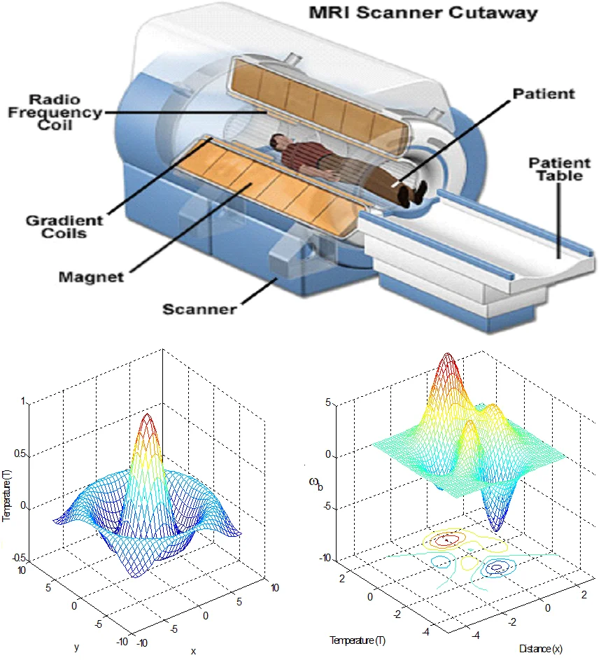
During the biological muscles (see Fig. 1), the temperature evaluation can be obtained in the context of the Penne’s bioheat equation, which is:

where, $T$, $\rho$, $C_T$ and $k$ represent the temperature distribution, the density of human tissue, the heat capacity of human tissue, the blood flow diffusion respectively. $C_b$ refers to the blood heat capacity, ${\omega }_b$ represents the blood flow perfusion, ${\rho }_b$ expresses the density of human blood. On the other hand, $T_b$, $Q$ and $\tau$ express the arterial blood temperature, the absorbed power density and relaxation time respectively.

3. Magnetic field equations

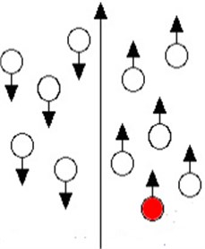
We consider rectangular coordinate system $\left(x,y,z\right)$ having origin on the surface $z=$ 0 and $z$-axis pointing vertically into the muscles. A magnetic field with constant intensity $H=(\mathrm{0,0},H_0)$ acts parallel to the bounding plane (table as the direction of the $z$-axis (Fig. 2)). Due to the application of initial magnetic field $H$, there are results of an induced magnetic field $h$ and an induced electric field $E$. The simplified linear equations of electrodynamics of slowly moving medium for a homogeneous,

Thermally and electrically conducting viscoelastic medium is:

where $\dot{u}$ is the partied velocity of the muscles, and the small effect of temperature gradient on $J$ is ignored. The dynamic displacement vector is actually measured from a steady state deformed position and the deformation is supposed to be small.

Fig. 1Geometry of the problem

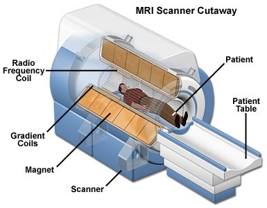
Fig. 2The direction of magnetic field

The components of the magnetic intensity vector in the viscoelastic (blood in muscles) medium are:

The electric intensity vector is normal to both the magnetic intensity and the displacement vectors. Thus, it has the components:

The current density vector $J$ be parallel to $E$, thus:

If we restrict our analysis to plane parallel to $xy$-plane with displacement vector (distance between cells in tissue) $u=(u,v,0)$. Body couples and heat sources can be written in visco-elasticity tissue by following the equations given by Minagawa et al. [1981], Green Lindsay [1972] and Othman and Baljeet [2007] as:

Introducing potential functions defined by:

The field Eqs. (10)-(11), we can reduce to:

where $\gamma =\left(3\lambda +2\mu +k\right){\alpha }_T$, ${\alpha }_T$ is coefficient of linear expansion, $\lambda$, $\mu$ and $k$ are representing effect of viscosity constants, $t$ is the time, $H$ is the initial uniform magnetic intensity vector, $h$ is the induced magnetic field vector, $E$ is the induced electric field vector, ${\mu }_0$ = $1/\left[2\right(1+\nu \left)\right]$ is magnetic permeability, ${\epsilon }_0$ is the electric permeability, $E_0$ is a constant modulus of visco-elasticity, $e={\nabla }^2\phi$ and ${\nabla }^2=\frac{{\partial }^2}{\partial x^2}+\frac{{\partial }^2}{\partial y^2}$.

The following dimensionless parameters were defined as:

where $\omega *=\frac{{\rho }_{b}C*C_0^2}{K*}$, $C_A^2=\frac{{\mu }_0{H}_0^2}{{\rho }_b}$, $\alpha =1+\frac{{\mu }_0^2{H}_0^2\epsilon }{{\rho }_b}$ and $L$ is the tissue length.

Eqs. (13) and (14) take the following form (dropping the dashed for convenience):

The dimensional form of Eq. (1) can be obtained as:

4. The normal mode analysis

The normal mode technique is used to solve Eq. (1) as:

where, $a$ is the wave number in the $y$-direction, $\omega$ is a complex time constant, ${\phi }^{*}\left(x\right)$, $q^{*}\left(x\right)$, ${\theta }^{*}$ and $G_0$ are the amplitude of the functions $\psi$, $\phi$, $\theta$ and $G$ respectively.

Substituting from Eqs. (21) into Eqs. (17), (18) and (20) we obtain:

where $m^2=a^2+p_f+\omega (1+\tau \omega )$, $n^2=a^2+\frac{\alpha {\omega }^2}{1+R_H+\widehat{R}}$,$n_1=\frac{1+\tau \omega }{1+R_H+\widehat{R}}$ and $s^2=a^2+\frac{4\alpha {\omega }^2}{3\widehat{R}}$.

Eliminating ${\theta }^{*}\left(x\right)$ between Eqs. (22) and (24), we get the following fourth order ordinary differential equation satisfied by ${\phi }^{*}\left(x\right)$:

where:

Eq. (25) can be factorized as:

where $k_j^2$, $j=1,2$ are the roots of the following characteristic equation:

The solution of Eq. (28) is given by:

In a similar manner, we get:

where $R_j(a,\omega )$ are parameters depending on $a$ and $\omega$.

The solution of Eq. (23) has the form:

Then, since:

Using Eqs. (30) and (32), in order to obtain the amplitude of the displacement components $u$ and $v$, which are bounded as $x\to \infty$, then Eqs. (33) and (34) become:

5. Boundary conditions

The plane boundary subjects to an instantaneous normal point force and the boundary surface is isothermal, the boundary conditions at the vertical plan $z=0$ and in the beginning of the operation of acting magnetic field at $x=0$ are (Othman and Lotfy 2011):

Using Eqs. (13), (16), on the non-dimensional boundary conditions and using Eqs. (37), (38), (39), we obtain the expressions of displacements and temperature distribution for the body under the effect radiation of magnetic field as follows:

where $r_1=(k_1^2-n^2)/n_1$, $r_2=(k_2^2-n^2)/n_1$.

Invoking the boundary conditions Eqs. (37-39) at the surface $x=0$ of the plate, we obtain a system of three equations. After applying the inverse of matrix method, we have the values of the four constants $R_j$, $j=\mathrm{1,2},3$. Hence, we obtain the expressions of displacements, and temperature distribution for the muscles:

where $S_1={\theta }_0^{*}-\frac{n^2(1+\tau \omega )G_0}{b_2}$ and $S_2=\frac{ia{n}_1(1+\tau \omega )G_0}{b_2}$.

6. Computational results

The properties of typical tissue and blood are used in these calculations as follow: ${\theta }_0^{*}=$ 0.01, $\rho =$ 1000 Kg/m³, $C_b=$ 4200 J/Kg° C, $T_b=$ 0.01, $k=$ 0.5 W/mC, ${\omega }_b=$ 0.5 Kg/m³ s, $j=$0.2×10^-15 cm³, $\lambda =$ 9.4×10¹¹ dyne/cm², $\mu =$ 4.0×10¹¹ dyne/cm², $a=2$, $t=$ 0.1.

On the other hand, the parameter values of this problem are taken in dimensionless which can be given by $G_0$ = 1.0, $T_b=$ 0.01, and the dimension of tissue is 3 cm. Fig. 3 displays the distribution of temperature at different three values of times against the distance. In this figure notice that the temperature distributions in tissue at the early stage of heating decreases with increasing the depth of tissue. The soft tissue can be considered as a viscous liquid for ultrasound propagation. The amount of heat which it is generated in the human tissue is more dependent on the tissue absorption coefficient. Acoustic absorption is due to the shear relaxation invariably cannot be accounted for by one relaxation time instead a distribution in continuous form of thermal memories must be used. In this case, this cause the relaxation process arises from the finite time taken for molecules to diffuse between adjacent shearing layers in the medium. Fig. 4 show the horizontal displacement distribution $u$ (distance between cells in the tissue) at different times as function of propagation distance. From this figure it can seen that the displacement distribution of tissue increases sharp in the start when the magnetic field acting on the tissue and hence smooth decreasing and converge to zero value (stable state) with the increase of the distance, after some time the displacement distribution more equilibrium this illustrated from the figure.

Fig. 3Temperature distribution as function of distance for different times (k= 0.5 W/m°C, ωb= 0.5 Kg/m3s)

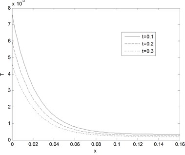
Fig. 4Horizontal displacement distribution u as function of distance for different times (k= 0.5 W/m°C, ωb= 0.5 Kg/m3s)

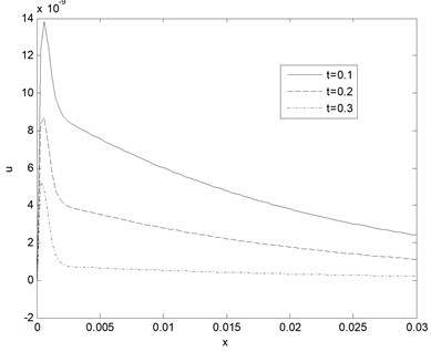
Fig. 5Vertical displacement distribution u as function of distance for different times (k= 0.5 W/m°C, ωb= 0.5 Kg/m3s)

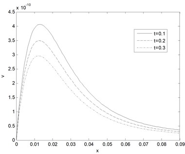
Fig. 6Temperature distribution as function of distance for different values of relaxation time (k= 0.5 W/m°C, ωb= 0.5 Kg/m3s)

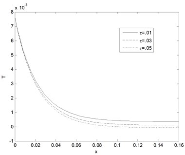
Fig. 5 show the vertical displacement distribution $v$ at various times which it taken as a function of distance propagation. From this figure the displacement distribution of tissue increases to arrive the maximum value (due to the magnetic field) in the start and hence smooth decreasing and converge to zero value (stable state) with the increase of the distance, after some time the displacement distribution more equilibrium. Fig. 6 displays the distribution of temperature at various dimensionless relaxation time as function of propagation distance. It can be seen that the temperature of tissue decreases with the increase of the thermal memories.

Fig. 7Horizontal displacement distribution u as function of distance for different values of relaxation time (k= 0.5 W/m°C, ωb= 0.5 Kg/m3s)

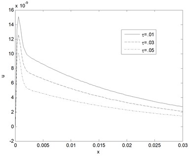
Fig. 8Vertical displacement distribution v as function of distance for different values of relaxation time (k= 0.5 W/m°C, ωb= 0.5 Kg/m3s)

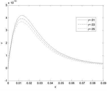
Fig. 9Effect of blood perfusion levels on temperature response as function of distance (k= 0.5 W/m°C, t= 0.1)

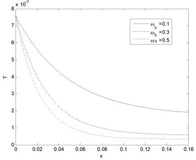
Fig. 10Effect of blood perfusion levels on Horizontal displacement u response as function of distance (k= 0.5 W/m°C, t= 0.1)

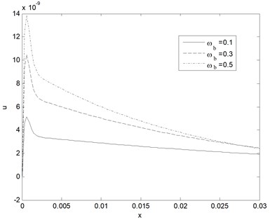
Fig. 7 shows horizontal displacement distribution $u$ at various dimensionless thermal memories which taken as a function of distance propagation. It can seen that the distance between the cell in tissue sharp increases in the first rang and then smooth decreases with the increase of the distance and converge to zero value when distance increases. Also, the amplitudes horizontal displacement decreases with the increase of the relaxation time. Fig. 8 shows vertical displacement distribution v at different non-dimensional relaxation time as function of propagation distance. From this figure it can seen that the distance between the cell in tissue smooth increases in the first rang and then smooth decreases also with the increase of the distance and converge to zero value when distance increases. Also, the amplitudes horizontal displacement decreases with the increase of the thermal memories. Fig. 9 displays the temperature of tissue responses corresponding to three various blood perfusion levels. For the case of ${\omega }_b=$0.5 Kg/m³s, the tissue temperature appears much smaller than that of using ${\omega }_b=$0.3 Kg/m³s at the same position. It can be seen that large blood perfusion tends to prevent the biological body from burn injury. Fig. 10 shows the horizontal displacement distribution $u$ at different three different blood perfusion levels. It clear from this figure the displacement between the cells in tissue increasing with blood perfusion increases. Fig. 11 shows the vertical displacement distribution v at different three different blood perfusion levels. It clears from this figure the displacement between the cells in this direction in tissue decreases with blood perfusion increases (it called spasm).

Fig. 11Effect of blood perfusion levels on vertical displacement v response s function of distance (k= 0.5W/m°C, t= 0.1)

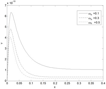
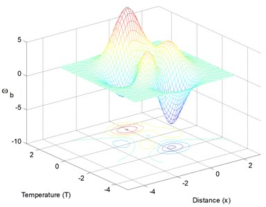
Fig. 12 shows the distribution of temperature in the human tissue, and depicted the surface tissue temperature and displacement increases immediately after the exposure, while in the deeper tissues, the temperature decreases slightly until after propagation in the $x$-$y$ plane. Fig. 13 depicts the tissue blood perfusion levels corresponding to the temperature responses and distance. The tissue temperature increases with the increase of the thermal conductivity of tissue It can be seen that large blood perfusion tends to prevent the biological body from burn injury.

Fig. 12Temperature distribution in 3-D (k= 0.5 W/m°C, ωb= 0.5 Kg/m3s, t= 0.1)

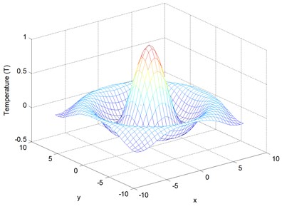
Fig. 13Effect of temperature response on blood perfusion levels as function of distance (k= 0.5 W/m°C, t= 0.1)

7. Conclusions

Effects of the individual’s physiological variables (such as blood perfusion, thermal conductivity and relaxation time) were investigated in detail. The present solution in this paper is very useful for a variety of bio-thermal studies. The curves in the context of the theories decrease or increase exponentially with increasing $x$, this indicate that the thermoelastic waves are unattenuated and nondispersive, where purely thermoelastic waves undergo both attenuation and dispersion. The presence of magnetic field plays a significant role in all the physical quantities. Analytical solutions based upon normal mode analysis for themoelastic problem in solids have been developed and utilized. The value of all the physical quantities converges to zero with an increase in distance $x$ and all functions are continuous. The numerical results using normal mode analysis are in a good agreement with previously published data. Indeed, the most important factor is the extent to penetrate the magnetic field and the arrival of magnetic energy into the cells of the body in the areas sought to be accessed, and the duration of exposure to the magnetic field is very important, as the intensity of penetration of the field directly related to the mass of material magnetic-generating field and how to focus the magnetic field and treatment domain magnetic helps to get rid of pain in general also helps diabetics to lower blood sugar and cholesterol in the blood and reduce the swelling and works to calm the nervous system