Abstract
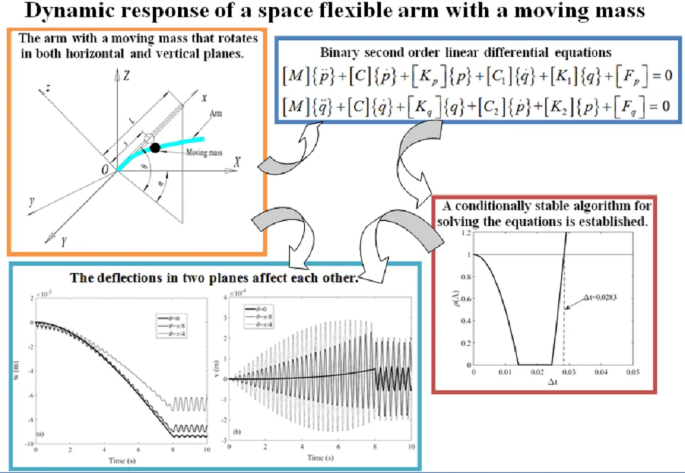
The dynamic characteristic of a space rotating flexible arm with moving mass were investigated. The space arm with moving mass can rotate around the fixed end in horizontal and vertical planes simultaneously. And the lateral deflections of the arm in the two planes were considered. The equations of the structure were derived by the Lagrange’s equation with the assumed mode method. And a system of binary second order linear differential equations is gotten. Based on the central difference method, a conditionally stable algorithm for solving the equations is established. Due to the coupling of lateral displacements of the arm in horizontal and vertical planes, the increase of the angular velocity in one plane will increase the lateral displacements in the other plane. When the angle between the arm and the horizontal plane increases, the component of gravity along the normal direction of the beam will decrease, resulting in a decrease in lateral displacements in vertical plane, however, it will lead to a decrease in stiffness in horizontal plane and thus an increase in lateral displacements. Compared with moving mass, moving load ignores the influence of inertial force, so the calculation results of moving mass and moving load are different. The conclusions provide calculation basis for the design of similar structures.
Highlights
- The governing equation is a set of binary second-order linear differential equations
- The algorithm established for solving the equations is conditionally stable
- The deflections in two planes affect each other
1. Introduction
The vibration of structures under moving mass or moving load is an important engineering problem, such as a bridge with travelling vehicles and a robotic arm carrying a moving end effecter. Because of the importance of such problems in engineering, it has attracted the attention of many researchers in the last few decades. There are a lot of works can be found in the published literature.
In most studies, the structures are considered to be no rotating. Wu [1] investigated the dynamic response of an inclined beam excited by moving mass and the moving mass element is used in his analysis. Yang et al. [2] presented an analytical study on the free and forced vibration of inhomogeneous Euler–Bernoulli beams containing open edge cracks, and the beam is subjected to an axial compressive force and a concentrated transverse load moving along the longitudinal direction. Under different boundary conditions, Kiani et al. [3] gave a comprehensive assessment of design parameters for various beam theories subjected to a moving mass. A non-linear viscoelastic foundation supported finite Euler-Bernoulli beam with moving mass is studied by Ansari et al. [4], and the Galerkin method is used to discretize the non-linear partial differential equation of motion. Esen [5] investigated the dynamic behavior of a beam carrying accelerating mass. Then He [6] presented a modified finite element method that can be used to analyze the transverse vibrations of a Timoshenko beam subjected to a variable-velocity moving mass. Nikkhoo et al. [7] proposed a new orthogonal basis for the spatial discretization tracking the dynamic response of shear deformable beams with moving mass. Uzzal et al. [8] presented the dynamic response of an Euler-Bernoulli beam supported on two-parameter Pasternak foundation subjected to moving load as well as moving mass. Wang et al. [9] developed a high-order shear deformable beam model and investigated the transient response of a sandwich porous beam when acted upon by a non-uniformly distributed moving mass. Jena, Parhi and other authors [10-15] studied cracked structures subjected to moving mass problems. Besides, Parida, Jena and others [16-21] investigated the dynamic and static problems of composite structures.
The problem becomes more difficult if the structures rotate about an axis. For a rotating structure with moving mass, the interaction between rigid and flexible body motions is highly demanded. Some of the researchers studied the dynamic response of rotating shaft subject to moving mass or moving load. Different beam theories are employed to model the rotating shaft with a moving load by Katz et al. [22]. Lee [23] analyzed dynamic response of a rotating shaft subject to axial force and moving loads by using Timoshenko beam theory and the assumed mode method. Shiau [24] investigated the dynamic response of a rotating multi-span shaft with general boundary conditions subjected to an axially moving load. Other researchers studied the dynamic responses of structures rotating in a plane and exited by moving mass or moving load. Choura [25] investigated the reduction of residual vibrations for the position control of a flexible rotating beam carrying a payload mass. Fung and Yau [26] studied the vibration frequencies of a clamped-free flexible beam rotating in a horizontal plane and carrying a moving mass. And they [27] derived the equation of motion of the system which took into account the effect of centrifugal stiffening due to the rotation of the beam. Ouyang and Wang [28] presented a dynamic model for the vibration of a rotating Timoshenko beam subjected to a three-directional load moving in the axial direction. Lv et al. [29] developed a Fourier Spectral method (FSM) for the vibration analysis of a rotating Rayleigh beam exited by moving force.
To the author's knowledge, arm with a moving mass that rotates in both horizontal and vertical planes has not been reported. In this problem, the rotation motion of the arm in one plane will affect the deflection in the other. In order to find out the influence of the rotating motion of the beam in two planes on the deflections, this study is done. The dynamic equation of the structure is a system of binary second-order linear differential equations. Based on the central difference method, an algorithm is designed to solve the coupled equations. The influences of the rotation motion of the arm in two planes and the influences of the angle between the arm and the horizontal plane on the deflection in two planes were studied. In addition, the influences of moving mass and moving load on the deflection of the arm were compared.
2. Formulation of the equations of motion
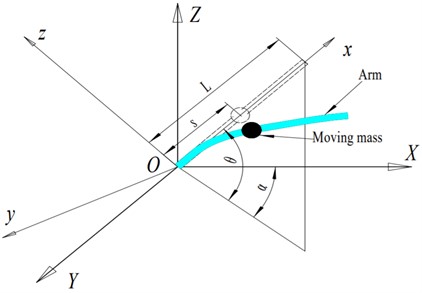
A uniform space rotating flexible arm with a moving mass is displayed in Fig. 1. is the global reference frame, while is the rotating reference frame. The fixed end of the arm is located at point and the axis is directed along the undeformed configuration of the arm. The Angle between the -axis and the plane is denoted as . In this studying, 0 /2 is considered. The angular displacement of the arm rotates about axis is denoted as . The moving mass moves along the arm. The length of the arm is , is the displacement of the moving mass in the direction while and are the velocity and acceleration of the moving mass relative to the arm respectively.
The global position of an arbitrary material point on the arm can be expressed as:
where is the rotational transformation matrix from the rotating coordinate system to the fixed reference frame . It can be expressed as:
where:
are the rotational transformation matrices of the coordinate system rotating about the axis and the axis respectively. is the location of the point in the rotating coordinate system and can be written as:
where and are the lateral displacements along and axis respectively. The velocity of the point is:
Fig. 1A space rotating flexible arm with moving mass
The kinetic energy of the arm can be written as:
where , and are the mass density, cross sectional area and the rotational inertia of the arm respectively. Based on Euler-Bernoulli beam theory [30], the elastic potential energy of the arm are given by:
where is the modulus of elasticity, and are the moment of inertia of arm section to z axis and axis respectively. And the gravitational potential energy is:
The axial inertial force consists of centrifugal force [27] and gravity can be written as:
Thus, potential energy generated by can be written as:
Now, let us consider the kinetic energy and potential energy of the moving mass. The location of the moving mass in the rotating coordinate system can be written as:
and the velocity is:
Thus, the velocity of the moving mass in the fixed reference frame is expressed as:
For a concentrated moving mass, the kinetic energy is:
The gravitational potential energy can be written as:
The total kinetic energy and potential energy of the system can be expressed as:
Lagrange’s equation with the assumed mode method is used to determine the equation of motion of the structural system. To use the assumed mode method, the flexible displacements of the arm can be expressed in terms of the generalized coordinates and displacement shape functions:
where , and . For cantilevered beam, the shape functions are:
where is obtained from the following characteristic equation:
Lagrange’s equation is written as:
Substituting the energy expressions into Eq. (22), the equations of motion of the whole structural system are gotten:
where:
3. Solution of the equations
3.1. Method
In this study, the central difference method is employed to solve the equations. Let , … be a partition of the time domain (0, ), the time step is . Then at each discrete time point , {} and {} can be expressed as and respectively. According to the central difference method, the velocity and acceleration can be expressed as [31]:
At each time point , the governing equations can be expressed as:
Substituting Eq. (25) and (26) into Eq. (27) and (28) respectively, we will get:
where:
Upon rearranging Eq. (29), we obtain the following equation:
Then, substituting Eq. (31) into Eq. (30) yields:
where , .
By solving Eq. (32), we can get . Then can be obtained by Eq. (31).
The initial conditions of displacement and velocity are given as follows:
By the governing equations, the initial acceleration is:
According to the central difference algorithm, we can get:
Eliminating and in the above two formulas, we will get:
The solving procedure is summarized in Table 1.
Table 1Implementation of the algorithm
A. Data input and initialization (a) Set initial values:, , , (b) Form coefficient matrices: [], [], [], [], [], [], [], [], [] (c) Compute initial accelerations: and (d) Compute and . B. For each time interval () (a) Form coefficient matrices: [], [], [], [], [], [], [], [], [] (b) Form effective matrices: [], [], {}, {} – Compute effective stiffness matrix: – Compute effective external force vectors: (c) Solve equations: (d) Update solutions: , , , , If go to (a), else terminate |
3.2. Stability
To analyze the stability of the method we consider a single-degree-of-freedom (SDOF) system [32]:
The stability can be evaluated with the solution succinctly written in the recursive form [31, 32]:
and the amplification matrix is expressed as:
where , , , , , , The stability of an algorithm depend upon the eigenvalues of the amplification matrix. The stability condition is [31, 32]:
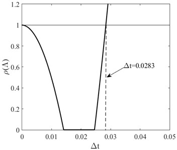
where is the spectral radius of which is defined as , and are the eigenvalues of . In this analysis, 1, 1, 1, 5000, 5000, 1, 1. The value of is plotted against in Fig. 2. It can be seen that when , the algorithm is stable. Thereby, it is a conditionally stable algorithm.
Fig. 2Spectral radius of the amplification matrix.
4. Numerical simulation
4.1. Validation
In order to validate the equations of motion and computer program in this paper, comparisons with the results available in the open literature are made. A flexible arm with moving mass rotates in a horizontal plane about axis is considered in [27]. Therefore , and in the program are all zero. To be consistent with [27], the non-dimensional parameters are defined as follows:
and are given by:
where:
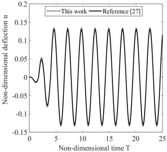
and and are the initial and final position of the moving mass with reference to the axes respectively, and is the traveling time of the mass. In this simulation, the mass moves towards the free end from (0.025, 0.2) to (0.8, 0.1), and other parameters are 0.5, 25, and 5. Non-dimensional deflections of arm under the moving mass are shown in Fig. 3. It is observed that the deflection obtained by the present work is in good agreement with that of Ref. [27].
Fig. 3Non-dimensional deflection of arm under the moving mass
4.2. Simulation examples
A uniform space rotating flexible arm with a moving mass as Fig. 1 is considered. The material of the arm is steel, which 209 GPa, 7800 kg/m3. The dimensions of the system are 2 m, 1.33×10⁻⁸ m4, 4×10⁻⁴ m2, and the moving mass 1 kg. In the following analysis, we take = 0.001.
First, three cases are used to study the influence of the rotating motion in horizontal and vertical planes on the lateral displacements. The mass moves towards the free end from the fixed end, and the initial conditions are: 0, = 0, = 0, 0, = 0, = 0. The movement rules of the system are given as follows:
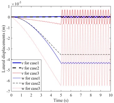
The arm rotates in the horizontal plane in case1 while it rotates in the vertical plane in case 2, and it rotates both in horizontal and vertical planes in case 3. After the travelling time passed (5), there is no mass and arm motion in the three cases. Fig. 4 shows the lateral displacements ( and ) of free end of the arm in horizontal and vertical plane. It can be observed from Fig. 4 that the lateral displacements of case3 are larger than that of case1 and case 2. That is to say, under the same conditions, compared with rotating motion of the arm only in one plane (horizontal or vertical plane), rotating motion of the arm in the other plane at the same time will increase the lateral displacements in both planes. This is due to the coupling of lateral displacements in the two planes.
Fig. 4Lateral displacements of arm under the moving mass in case 1, 2 and 3
Next, the influence of the angle between the arm and the horizontal plane and the rotation acceleration of the arm on the lateral displacement is investigated. In case 4, the mass still moves from the fixed end to the free end, and the movement rules of the system are given as follows:
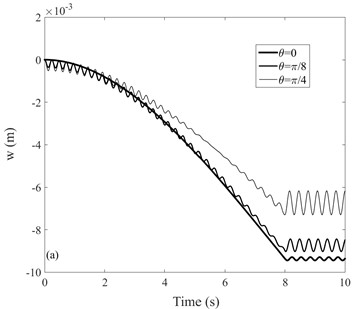
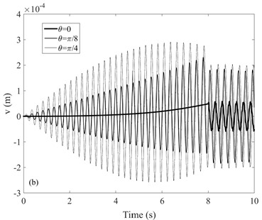
The arm rotates around the axis with a constant angular velocity, and let be 0, and respectively. The initial conditions are: 0, = 0, 0, = 0, = 0. The lateral displacements of free end of the arm are shown in Fig. 5. The transverse component of gravity of the moving mass decreases with the increase of . Thereby, it can be seen clearly from Fig. 5(a) that in the steady state vibration phase (8 s) the tip lateral displacements decrease with the increase of . This is caused by the decrease of the component force of gravity along the normal direction of the arm. However, the tip lateral displacements increase with the increase of . According to Eq. (24), the increase of will cause the decrease of stiffness matrix []. Therefore, the lateral displacements increases accordingly.
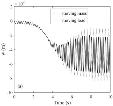
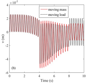
Finally, comparison between moving load and moving mass responses is carried out. In case 8 the mass moves from the fixed end to the free end, first with constant acceleration and then with constant deceleration. The initial and final velocities of the mass are both 0. The angular velocities of the arm in both horizontal and vertical plane also experienced a process of uniform increase at first and then uniform decrease, and their initial and final values are also 0. The dynamic responses of the arm under both moving load and moving mass conditions are considered. It can be observed from Fig. 6 that in the steady state vibration phase (8 s), the lateral displacement of moving mass is larger than that of moving load while the lateral displacement of moving load is larger than that of moving mass:
Fig. 5Lateral displacements of arm under the moving mass in case 4
a)
b)
Fig. 6Lateral displacements of arm under the moving mass in case 5
a)
b)
5. Conclusions
The problem of a space rotating flexible arm with a moving mass is investigated in this study. One end of the arm is fixed at the coordinate origin. The arm can rotate in both horizontal and vertical planes, and the lateral displacement in both planes is considered. The assumed mode method conjunction with Lagrange’s equation is used to derive the equations of the system. Then a set of coupled equations about the lateral displacements in the horizontal and vertical planes is obtained. Based on the central difference method, an algorithm is designed to solve the coupled equations. By numerical analysis, the following conclusions can be drawn:
1) The algorithm designed in this paper for solving binary second-order linear differential equations is a conditionally stable algorithm.
2) Due to the coupling of lateral displacements of the arm in horizontal and vertical planes, the increase of the angular velocity in one plane will increase the lateral displacements in the other plane.
3) When the angle between the arm and the horizontal plane increases, the component of gravity along the normal direction of the beam will decrease, resulting in a decrease in lateral displacements , however, it will lead to a decrease in stiffness in horizontal plane and thus an increase in lateral displacements .
4) Compared with moving mass, moving load ignores the influence of inertial force, so the calculation results of moving mass and moving load are different. In the steady state vibration phase, the lateral displacement w of moving mass is larger than that of moving load while the lateral displacement of moving load is larger than that of moving mass.
References
-
J.-J. Wu, “Dynamic analysis of an inclined beam due to moving loads,” Journal of Sound and Vibration, Vol. 288, No. 1-2, pp. 107–131, Nov. 2005, https://doi.org/10.1016/j.jsv.2004.12.020
-
J. Yang, Y. Chen, Y. Xiang, and X. L. Jia, “Free and forced vibration of cracked inhomogeneous beams under an axial force and a moving load,” Journal of Sound and Vibration, Vol. 312, No. 1-2, pp. 166–181, Apr. 2008, https://doi.org/10.1016/j.jsv.2007.10.034
-
K. Kiani, A. Nikkhoo, and B. Mehri, “Prediction capabilities of classical and shear deformable beam models excited by a moving mass,” Journal of Sound and Vibration, Vol. 320, No. 3, pp. 632–648, Feb. 2009, https://doi.org/10.1016/j.jsv.2008.08.010
-
M. Ansari, E. Esmailzadeh, and D. Younesian, “Internal-external resonance of beams on non-linear viscoelastic foundation traversed by moving load,” Nonlinear Dynamics, Vol. 61, No. 1-2, pp. 163–182, Jul. 2010, https://doi.org/10.1007/s11071-009-9639-0
-
I. Esen, “Dynamic response of a beam due to an accelerating moving mass using moving finite element approximation,” Mathematical and Computational Applications, Vol. 16, No. 1, pp. 171–182, Apr. 2011, https://doi.org/10.3390/mca16010171
-
I. Esen, “Dynamic response of a functionally graded Timoshenko beam on two-parameter elastic foundations due to a variable velocity moving mass,” International Journal of Mechanical Sciences, Vol. 153-154, pp. 21–35, Apr. 2019, https://doi.org/10.1016/j.ijmecsci.2019.01.033
-
A. Nikkhoo, A. Farazandeh, and M. Ebrahimzadeh Hassanabadi, “On the computation of moving mass/beam interaction utilizing a semi-analytical method,” Journal of the Brazilian Society of Mechanical Sciences and Engineering, Vol. 38, No. 3, pp. 761–771, Mar. 2016, https://doi.org/10.1007/s40430-014-0277-1
-
R. U. A. Uzzal, R. B. Bhat, and W. Ahmed, “Dynamic response of a beam subjected to moving load and moving mass supported by Pasternak foundation,” Shock and Vibration, Vol. 19, No. 2, pp. 205–220, 2012, https://doi.org/10.3233/sav-2011-0624
-
Y. Wang, A. Zhou, T. Fu, and W. Zhang, “Transient response of a sandwich beam with functionally graded porous core traversed by a non-uniformly distributed moving mass,” International Journal of Mechanics and Materials in Design, Vol. 16, No. 3, pp. 519–540, Sep. 2020, https://doi.org/10.1007/s10999-019-09483-9
-
S. P. Jena, D. R. Parhi, and D. Mishra, “Comparative study on cracked beam with different types of cracks carrying moving mass,” Structural Engineering and Mechanics, Vol. 56, No. 5, pp. 797–811, Dec. 2015, https://doi.org/10.12989/sem.2015.56.5.797
-
S. P. Jena and D. R. Parhi, “Response analysis of cracked structure subjected to transit mass – a parametric study,” Journal of Vibroengineering, Vol. 19, No. 5, pp. 3243–3254, Aug. 2017, https://doi.org/10.21595/jve.2017.17088
-
D. R. Parhi and S. P. Jena, “Dynamic and experimental analysis on response of multi-cracked structures carrying transit mass,” Proceedings of the Institution of Mechanical Engineers, Part O: Journal of Risk and Reliability, Vol. 231, No. 1, pp. 25–35, Feb. 2017, https://doi.org/10.1177/1748006x16682605
-
S. P. Jena and D. R. Parhi, “Response of damaged structure to high speed mass,” Procedia Engineering, Vol. 144, pp. 1435–1442, 2016, https://doi.org/10.1016/j.proeng.2016.05.175
-
S. P. Jena and D. R. Parhi, “Dynamic response and analysis of cracked beam subjected to transit mass,” International Journal of Dynamics and Control, Vol. 6, No. 3, pp. 961–972, Sep. 2018, https://doi.org/10.1007/s40435-017-0361-3
-
S. P. Jena and D. Parhi, “Structural damage detection in moving load problem using JRNNs based method,” Journal of Theoretical and Applied Mechanics, No. 3, pp. 665–676, 2019.
-
P. C. Jena, D. R. Parhi, and G. Pohit, “Dynamic study of composite cracked beam by changing the angle of bidirectional fibres,” Iranian Journal of Science and Technology, Transactions A: Science, Vol. 40, No. 1, pp. 27–37, 2016, https://doi.org/10.1007/s40995-016-0006-yissn
-
P. C. Jena, D. R. Parhi, and G. Pohit, “Fault Measurement in Composite Structure by Fuzzy-Neuro Hybrid Technique from the Natural Frequency and Fibre Orientation,” Journal of Vibration Engineering and Technologies, Vol. 5, No. 2, pp. 124–136, 2017.
-
S. P. Parida, D. P. C. Jena, and D. R. R. Dash, “Dynamic analysis of laminated composite beam using Timoshenko beam Theory,” International Journal of Engineering and Advanced Technology, Vol. 8, No. 6, pp. 190–196, Aug. 2019, https://doi.org/10.35940/ijeat.e7159.088619
-
P. C. Jena, D. R. Parhi, and G. Pohit, “Dynamic investigation of FRP cracked beam using neural network technique,” Journal of Vibration Engineering and Technologies, Vol. 7, No. 6, pp. 647–661, Dec. 2019, https://doi.org/10.1007/s42417-019-00158-5
-
S. P. Parida and P. C. Jena, “Selective layer-by-layer fillering and its effect on the dynamic response of laminated composite plates using higher-order theory,” Journal of Vibration and Control, p. 107754632210811, Apr. 2022, https://doi.org/10.1177/10775463221081180
-
S. P. Parida, P. C. Jena, and R. R. Dash, “Dynamics of rectangular laminated composite plates with selective layer-wise fillering rested on elastic foundation using higher-order layer-wise theory,” Journal of Vibration and Control, p. 107754632211383, Nov. 2022, https://doi.org/10.1177/10775463221138353
-
R. Katz, C. W. Lee, A. G. Ulsoy, and R. A. Scott, “The dynamic response of a rotating shaft subject to a moving load,” Journal of Sound and Vibration, Vol. 122, No. 1, pp. 131–148, Apr. 1988, https://doi.org/10.1016/s0022-460x(88)80011-7
-
H. P. Lee, “Dynamic response of a rotating timoshenko shaft subject to axial forces and moving loads,” Journal of Sound and Vibration, Vol. 181, No. 1, pp. 169–177, Mar. 1995, https://doi.org/10.1006/jsvi.1995.0132
-
T. N. Shiau, K. H. Huang, F. C. Wang, and W. C. Hsu, “Dynamic response of a rotating multi-span shaft with general boundary conditions subjected to a moving load,” Journal of Sound and Vibration, Vol. 323, No. 3-5, pp. 1045–1060, Jun. 2009, https://doi.org/10.1016/j.jsv.2009.01.034
-
S. Choura, “Reduction of residual vibrations in a rotating flexible beam with a moving payload mass,” Proceedings of the Institution of Mechanical Engineers, Part I: Journal of Systems and Control Engineering, Vol. 211, No. 1, pp. 25–34, Feb. 1997, https://doi.org/10.1243/0959651971539669
-
E. H. K. Fung and D. T. W. Yau, “Vibration frequencies of a rotating flexible arm carrying a moving mass,” Journal of Sound and Vibration, Vol. 241, No. 5, pp. 857–878, Apr. 2001, https://doi.org/10.1006/jsvi.2000.3332
-
D. T. W. Yau and E. H. K. Fung, “Dynamic response of a rotating flexible arm carrying a moving mass,” Journal of Sound and Vibration, Vol. 257, No. 1, pp. 107–117, Oct. 2002, https://doi.org/10.1006/jsvi.2002.5033
-
H. Ouyang and M. Wang, “A dynamic model for a rotating beam subjected to axially moving forces,” Journal of Sound and Vibration, Vol. 308, No. 3-5, pp. 674–682, Dec. 2007, https://doi.org/10.1016/j.jsv.2007.03.082
-
B. Lv, W. Li, and H. Ouyang, “Moving force-induced vibration of a rotating beam with elastic boundary conditions,” International Journal of Structural Stability and Dynamics, Vol. 15, No. 1, p. 1450035, Jan. 2015, https://doi.org/10.1142/s0219455414500357
-
O. A. Bauchau and J. I. Craig, “Euler-Bernoulli beam theory,” Structural Analysis, pp. 173–221, 2009, https://doi.org/10.1007/978-90-481-2516-6_5
-
G. M. Hulbert, “Time finite element methods for structural dynamics,” International Journal for Numerical Methods in Engineering, Vol. 33, No. 2, pp. 307–331, Jan. 1992, https://doi.org/10.1002/nme.1620330206
-
B. Wu, H. Bao, J. Ou, and S. Tian, “Stability and accuracy analysis of the central difference method for real-time substructure testing,” Earthquake Engineering and Structural Dynamics, Vol. 34, No. 7, pp. 705–718, Jun. 2005, https://doi.org/10.1002/eqe.451
About this article

The authors have not disclosed any funding.
The datasets generated during and/or analyzed during the current study are available from the corresponding author on reasonable request.
The authors declare that they have no conflict of interest.
