Experimental study on stress wave propagation in jointed rock coupling the effect of JMC & JRC

Hong, Shengnan; Li, Haibo

doi:10.21595/vp.2022.22361

Vibroengineering Procedia

Browse Procedia

Published: 21 April 2022

Check for updates

Experimental study on stress wave propagation in jointed rock coupling the effect of JMC & JRC

Shengnan Hong¹

Haibo Li²

^{1, 2}State Key Laboratory of Geomechanics and Geotechnical Engineering, Institute of Rock and Soil Mechanics, Chinese Academy of Sciences, Wuhan, 430071, China

²University of Chinese Academy of Sciences, Beijing, 100049, China

Corresponding Author:

Shengnan Hong

Cite the article Download PDF

Downloads 356

Abstract

The objective of this study is to experimentally investigate how the rough joints effect the stress wave propagation through jointed rocks coupling the effect of the joint matching coefficient (JMC) and joint roughness coefficient (JRC). The Split Hopkinson Pressure Bar (SHPB) apparatus was adopted to conduct uniaxial compression experiments on jointed specimens. The joint matching coefficient (JMC) and joint roughness coefficient (JRC) are introduced as morphology parameters to estimate joint roughness. Based on SHPB experiments, we found out that the joint matching coefficient (JMC) has a greater influence on the transmission and reflection coefficient than the joint roughness coefficient (JRC). Jointed specimens with lower JMC and JRC make less energy transmitted through it and have a smaller transmission coefficient and bigger reflection coefficients. Also, the joint with lower JMC and JRC has less initial stiffness and greater maximum closure.

Experimental study on stress wave propagation in jointed rock coupling the effect of JMC & JRC

Highlights

The joint matching coefficient (JMC) and joint roughness coefficient (JRC) are introduced as morphology parameters to estimate joint roughness.
The finding that JMC has a greater influence on the transmission and reflection coefficient than JRC.
The finding that jointed specimens with lower JMC and JRC make less energy transmitted through it.

1. Introduction

Rock is one common engineering material. Its mechanical properties are significantly affected by the additional mechanical compliance that results from joints, fractures, or faults [1]. Studying the effect of joints on stress wave propagation helps with designing and building underground structures in fractured rock masses under dynamic loading, like an earthquake, explosion, etc.

The study of joints involves quantifying the roughness as a morphological parameter. Barton [2], and Barton and Choubey [3] proposed a joint roughness coefficient (JRC) to describe the surface roughness and gave a set of 10 typical roughness profiles whose JRC ranges from 0 to 20. However, it is too subjective to estimate the JRC by comparing the joint surface to 10 typical roughness profiles. Hence, Tse and Cruden [4] put forward an empirical equation to calculate JRC correlating with $Z_{2}$ (the root mean square of the first derivative of the profile) and SF (structure function). Then Yang [5] improved the equation introduced by Tse and Cruden considering the self-affinity transformation law. On the other hand, rough joints in nature may suffer from weathering, loading and thermal cycles, which may alter the surface of joints and cause mismatching. Clearly, the degree of matching cannot be represented by JRC. However, the matching degree does affect the mechanical properties of joints. Cook [1] found that the mechanical stiffness or compliance of joints depends primarily upon the area of contact between the two surfaces of a joint. Then, Zhao [6] and Zhao [7] proposed the joint matching coefficient (JMC) as an independent joint surface geometrical parameter, which equals the percentage of joint surfaces in contact. During an experimental investigation, it is found that JMC has a crucial impact on the aperture, normal closure, stiffness, shear strength, and hydraulic conductivity of the joints. The joint matching coefficient (JMC) is coupled with the joint roughness coefficient (JRC) to fully describe the geometrical properties of joints.

The subject of this study is to experimentally investigate how the rough joints effect the stress wave propagation coupling the effect of JMC & JRC. A series of jointed specimens with different JMCs and JRCs were made to conduct dynamic uniaxial compression experiments. Based on the experiment, the effect of joint roughness on stress propagation is analyzed and discussed.

2. Experiments

2.1. Experimental facilities

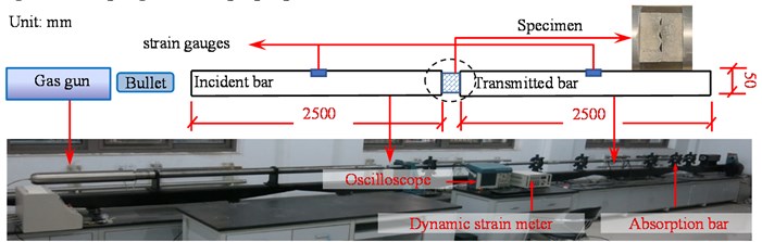
As shown in Fig. 1, the uniaxial compression test was conducted on the SHPB system. It consists of loading system, bar system, and measurement system. The loading system is a gas gun, which stores high-pressure nitrogen that pushes the bullet to move forward. The bar system contains four aluminum bars with the same circle cross-section (50 mm in diameter), namely bullet (250 mm in length), the incident bar (2500 mm in length), the transmitted bar (2500 mm in length), and the absorption bar (800 mm in length). In addition, the density $ρ$ and Young’s modulus $E$ of the aluminum bars are 2700 kg/m³ and 70 GPa, respectively. The measurement system is made up of dynamic strainmeter, oscilloscope, and two groups of strain gauges glued on the incident bar and transmitted bar.

Fig. 1The Split Hopkinson Pressure Bar (SHPB) test equipment

2.2. Specimen

We adopted the random fractal method suggested by to generate 3 different joint profile lines, whose JRCs are 1.1, 8.4 and 14.2. Based on three profile lines with different JRCs, we derived 4 different joint contact conditions by altering part of the profile lines in different degrees. So, we got 3 groups of designed jointed specimen models, the specimens in each group shared the same JRC but different JMCs, that is 1, 0.8, 0.6 and 0.4. Then we used 3-dimensional printed resin molds to cast cement specimens to control the shape of the specimen joint. Finally, here we got 12 jointed specimens with 3 kinds of JRCs and 4 kinds of JMCs, which are shown in Fig. 2. Each specimen is a cube (3 cm in height, 3.5 cm in length and width) that can be divided into 2 parts by an irregular surface, i.e., artificial joint.

The JRC of joint profile lines can be calculated from a commonly adopted empirical equation [5]:

1

J R C = 32.69 + 32.98 l o g_{10} Z_{2},

where the parameter $Z_{2}$ is given as:

2

Z_{2} = {[\frac{1}{m (Δ x)^{2}} \sum_{i = 1}^{m} (y_{i + 1} - y_{i})^{2}]}^{1 / 2} .

In this equation, $Δ x$ is the small constant horizontal distance between two adjacent points along the profile lines, $m$ denotes the number of points on the profile lines and is related to the ratio between cylindrical diameter $D_{s}$ and horizontal distance interval $Δ x$ , that is, $m = 1$ + integer ( $D_{s} / Δ x$ ). The ‘ $y_{i + 1} - y_{i}$ ’ denotes the amplitude difference between two adjacent points.

Fig. 2Specimens with different rough joints

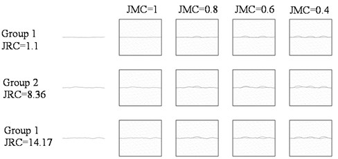
a) Designed jointed specimen cross sections

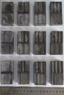
b) Actual test specimens with rough joint

3. Experiment data processing

According to the one-dimensional elastic stress wave theory, we can get the stress $σ$ , strain rate $\dot{ε}$ and strain $ε$ of the specimen according to the one-dimensional elastic stress wave theory, that is:

3

\dot{ε} (t) = \frac{C}{l} (ε_{i} (t) - ε_{r} (t) - ε_{t} (t)),

4

ε (t) = \frac{C}{l} \int_{0}^{t} (ε_{i} (t) - ε_{r} (t) - ε_{t} (t)) d t,

5

σ (t) = \frac{A}{2 A_{s}} E (ε_{i} (t) + ε_{r} (t) + ε_{t} (t)),

where $E$ is the elastic modulus of SHPB bars, $C$ is the stress wave velocity in bars, and $ε_{i} (t)$ , $ε_{r} (t)$ , $ε_{t} (t)$ are recorded strain datum of incident wave, reflected wave and transmitted wave, respectively. Where $l$ is the length of the specimen, $A$ and $A_{s}$ is the cross-section area of the bars and specimen, respectively.

Based on elastic theory, we can calculate the energy of stress waves, i.e. incident wave energy $E_{i} (t)$ , reflected wave energy $E_{r} (t)$ and transmitted wave energy $E_{t} (t)$ , as follows:

6

E_{i} (t) = A E c \int_{0}^{t} {ε_{i}}^{2} (t) d t, E_{r} (t) = A E c \int_{0}^{t} {ε_{r}}^{2} (t) d t, E_{t} (t) = A E c \int_{0}^{t} {ε_{t}}^{2} (t) d t .

Then we calculated the ratio of transmitted wave energy and reflected wave energy to incident wave energy, which is denoted as $T$ and $R$ , respectively. $T$ and $R$ can be expressed as:

7

T = \frac{m a x |E_{t} (t)|}{m a x |E_{i} (t)|}, R = \frac{m a x |E_{r} (t)|}{m a x |E_{i} (t)|} .

When we separate the deformation of intact cement ( $Δ v_{c}$ ) from jointed cement specimen ( $Δ v$ ), we get the joint closure ( $Δ v_{j}$ ):

8

Δ v_{j} = Δ v - Δ v_{c} .

4. Experiment results and analysis

4.1. Stress-strain curves of specimens

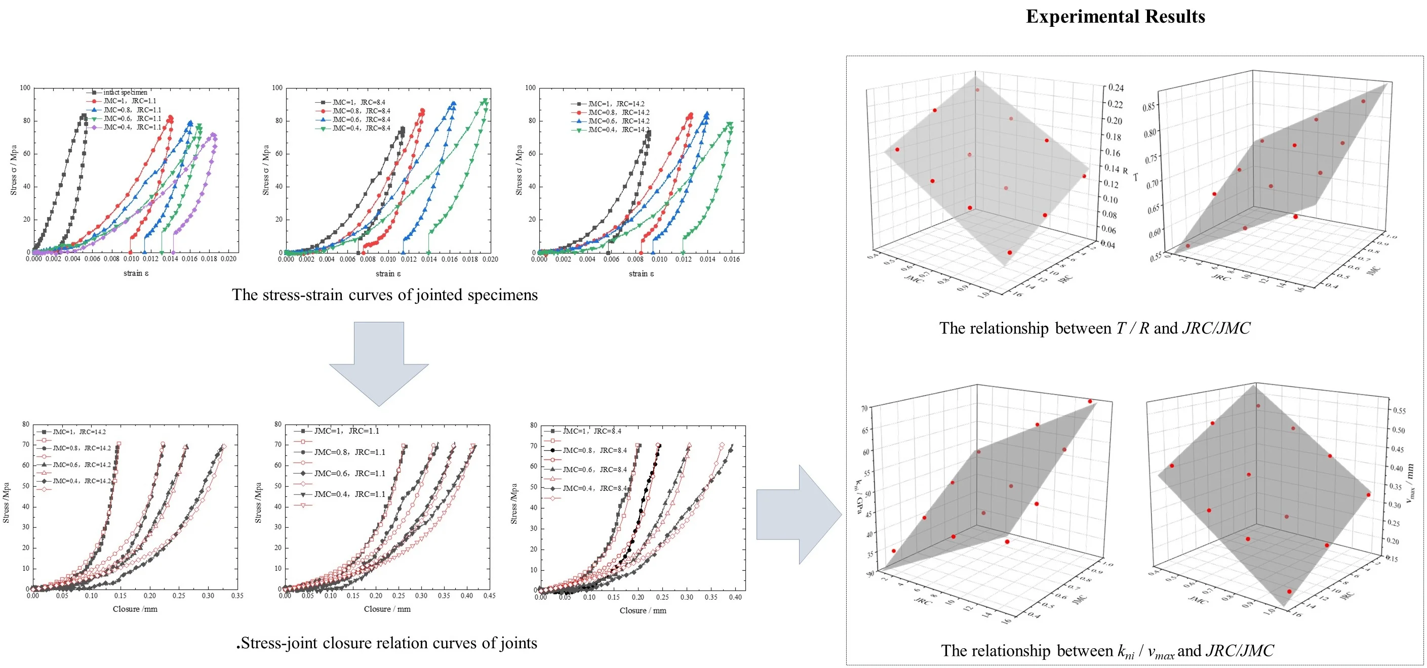
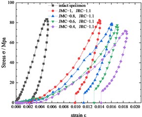
By Eqs. (4) and (5), we can obtain stress-strain relation curves of all specimens which are shown in Fig. 3 and 4. Different from jointed specimens, the intact specimen deforms much smaller than the jointed specimen under the similar level of stress. The deformation of the jointed specimen includes the deformation of the rock block itself and an additional weak interface, that is joint. And the deformation caused by joint is remarkable that accounts for a large proportion of the total deformation of the jointed specimen.

Fig. 3Comparing the stress-strain curves of jointed specimens with the same JMC but different JRC

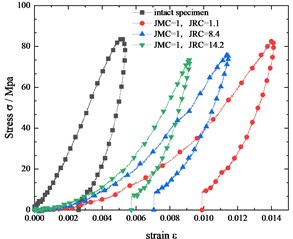
In Fig. 3, we compare the stress-strain curves of jointed specimens with the same JMC but different JRC. In specimen with the rougher joint surface is smaller than that of the jointed specimen with a flatter joint surface. Under the relatively low normal load, the rough joint surface is not broken and rougher joint surfaces have more contact area which contributes to a better interlocking of two parts of the jointed specimen. Besides, the rougher joint has more contact areas, which means lower pressure on joint surfaces under the same load. Naturally, the specimen with larger JRC deforms less than that with smaller JRC.

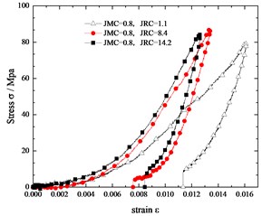
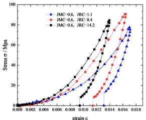
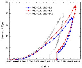
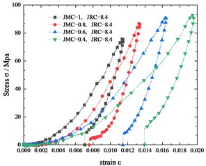
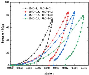
In Fig. 4, we compare the stress-strain curves of jointed specimens with the same JRC but different JMC. The curvature of the stress-strain curve increases with the JMC of the specimen. The deformation of the jointed specimen with a smaller JMC is larger than that of the jointed specimens with a larger JMC. It is easy to understand that the larger the JMC is, the larger the contact area is, the smaller the pressure will be, and the less deformation.

4.2. Transmission and reflection coefficients

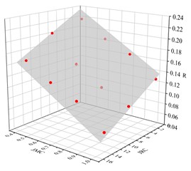
As we can see from the Fig. 3 and 4, specimens were performed at similar load levels. Therefore, the parameters derived from the originally test data are comparable. We calculated the stress wave transmission coefficient ( $T$ ) by Eq. (9) and the reflection coefficient ( $R$ ) by Eq. (10). Fig. 5 and 6 show the relationship between $T$ / $R$ and JMC/JRC. In Fig. 5 and 6, we can see that $T$ grows linearly with JMC and JRC, and $R$ decreases linearly with JMC and JRC. So, we adopt planes to fit them, that are:

9

T = 0.2622 \cdot J M C + 0.009344 \cdot J R C + 0.4553,

10

R = - 0.1538 \cdot J M C - 0.004886 \cdot J R C + 0.2876 .

Fig. 4Comparing the stress-strain curves of jointed specimens with the same JRC but different JMC

The goodness of the fits ( $R^{2}$ ) are 0.979 and 0.974, respectively. It means the equations above fits the test results quite well. The JMC ranges from 0 to 1, and the JRC ranges from 0 to 20. According to Eq. (12), $T$ changes about 0.2622 because of JMC and about 0.1869 because of JRC. According to Eq. (13), $R$ changes about 0.1538 because of JMC and about 0.0977 because of JRC. Hence, the JMC has more influence on the transmission coefficient than JRC. The jointed specimen with larger JMC and JRC has more stress wave energy passed through it and less energy reflected.

Fig. 5The relationship between T and JRC/JMC

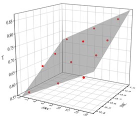
Fig. 6The relationship between R and JRC/JMC

4.3. The joint stiffness and maximum closure

To get the joint closure, we remove the cement block deformation from the total deformation of the jointed specimen using Eq. (11). Then, we can get the stress-closure relations of all joints, which are shown as black lines in Fig. 7.

The normal stress-closure expression of the B-B model [9] is commonly adopted to cope with the issue of joint mechanical properties, which is:

11

σ = \frac{k_{n i} \times Δ v_{j}}{1 - Δ v_{j} / v_{m a x}},

where $Δ v_{j}$ is the closure of the joint and the $v_{m a x}$ is the maximum closure of the joint. The $k_{n i}$ is the derivative of the stress-closure curves at the initial point.

Fig. 7Stress-joint closure relation curves

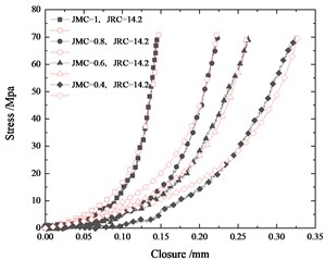
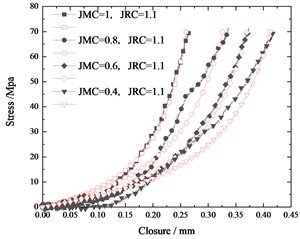
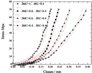
Fig. 8The relationship between kni and JRC/JMC

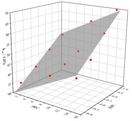
Fig. 9The relationship between vmax and JRC/JMC

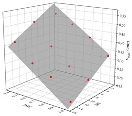
So we apply the Eq. (14) to fit the joint stress-closure curves. The fitting curves are shown as red lines in Fig. 7. The B-B model fits well with the stress-closure curves of joints. The variations of parameters ( $v_{m a x}$ and $k_{n i}$ ) obtained from curve-fitting with JRC and JMC are displayed in Fig. 8 and Fig. 9, respectively. Joint parameters ( $v_{m a x}$ and $k_{n i}$ ) are linearly correlated with JMC and JRC. In addition, $k_{n i}$ increases linearly with JRC and JMC, and $v_{m a x}$ decreases linearly with JRC and JMC. So, they are all fitted with the planes, which are displayed as follows:

12

k_{n i} = 34.43 \cdot J M C + 1.204 \cdot J R C + 17.52,

13

v_{m a x} = - 0.3828 \cdot J M C - 0.01287 \cdot J R C + 0.7162 .

5. Conclusions

The test results are displayed and discussed above. The conclusions are listed below:

1) Both JMC and JRC affect the propagation of stress waves through jointed specimens. Jointed specimens with higher JRC and JMC make more energy transmitted through the joint and less energy have a small transmission coefficient. Besides, we found that JMC has a greater influence on stress wave transmission through the specimen with the joint. Therefore, we should pay more attention to the contacting area of the joint on problems of stress wave propagation.

2) As for joint mechanical property, the joint maximum closure ( $v_{m a x}$ ) and initial stiffness ( $k_{n i}$ ) are two representative parameters, which can well describe the dynamic behavior of the joint. When JMC and JRC decreases, the $v_{m a x}$ would decrease and $k_{n}$ would increase.

References

Cook and N. G. W., “Natural joints in rock: Mechanical, hydraulic and seismic behaviour and properties under normal stress,” International Journal of Rock Mechanics and Mining Sciences and Geomechanics Abstracts, Vol. 29, No. 3, pp. 198–223, May 1992, https://doi.org/10.1016/0148-9062(92)93656-5

Publisher
N. Barton, “The shear strength of rock and rock joints,” International Journal of Rock Mechanics and Mining Sciences and Geomechanics Abstracts, Vol. 13, No. 9, pp. 255–279, Sep. 1976, https://doi.org/10.1016/0148-9062(76)90003-6

Publisher
N. Barton and V. Choubey, “The shear strength of rock joints in theory and practice,” Rock Mechanics Felsmechanik Mecanique des Roches, Vol. 10, No. 1-2, pp. 1–54, Dec. 1977, https://doi.org/10.1007/bf01261801

Publisher
R. Tse and D. M. Cruden, “Estimating joint roughness coefficients,” International Journal of Rock Mechanics and Mining Sciences and Geomechanics Abstracts, Vol. 16, No. 5, pp. 303–307, Oct. 1979, https://doi.org/10.1016/0148-9062(79)90241-9

Publisher
Z. Y. Yang, S. C. Lo, and C. C. Di, “Reassessing the joint roughness coefficient (JRC) estimation using Z2,” Rock Mechanics and Rock Engineering, Vol. 34, No. 3, pp. 243–251, Aug. 2001, https://doi.org/10.1007/s006030170012

Publisher
Zhao J., “Experimental studies of the hydro-thermo-mechanical behaviour of joints in granite,” University of London, 1987.

Search CrossRef
J. Zhao, “Joint surface matching and shear strength part A: joint matching coefficient (JMC),” International Journal of Rock Mechanics and Mining Sciences, Vol. 34, No. 2, pp. 173–178, Feb. 1997, https://doi.org/10.1016/s0148-9062(96)00062-9

Publisher
Xu et al., “Fractal simulation of joint profiles and relationship between JRC and fractal dimension,” Chinese Journal of Rock Mechanics and Engineering, Vol. 21, No. 11, pp. 1663–1666, 2002.

Search CrossRef
S. C. Bandis, A. C. Lumsden, and N. R. Barton, “Fundamentals of rock joint deformation,” International Journal of Rock Mechanics and Mining Sciences and Geomechanics Abstracts, Vol. 20, No. 6, pp. 249–268, Dec. 1983, https://doi.org/10.1016/0148-9062(83)90595-8

Publisher

About this article

Received

28 December 2021

Accepted

26 January 2022

Published

21 April 2022

SUBJECTS

Seismic engineering and applications

DOI

https://doi.org/10.21595/vp.2022.22361

Keywords

rock joint

stress wave

joint matching coefficient

joint roughness coefficient

Acknowledgements

The study was supported by the Chinese National Science Research Fund (Grant Nos. 41525009, 51439008) and the National Key R&D Program of China (2020YFA0711802).

This is an open access article distributed under the Creative Commons Attribution License, which permits unrestricted use, distribution, and reproduction in any medium, provided the original work is properly cited.

Previous article in issue Previous Next article in issue Next

Research article

2023 09 21

Experimental study on waterproof performance of assembled station joints of Shenzhen Rail Transit Line

Xianli Ding, Deyong Yu, Yongxiang Liu, Feiqi Ou, Yongzhong Deng, Qian Zhang, Mingyuan Du, Shujie Cao, Yixuan Zhao, Zihang Zhang, Yan Ma

Research article

2020 06 30

Impact compression properties of artificial cemented sand material under active confining pressure

Jinjin Ge, Ying Xu

Research article

2020 04 02

Study on anisotropic characteristics of dynamic deformation parameters of phyllite

Fu’an Si, Jiangbo Xu, Yilun Cui, Dongyang Fei, Kun Li

Research article

2019 06 30

Strength characteristics and failure behavior of ubiquitous-joint rock-like specimens under compressive-shear stress: experimental study and digital speckle correlation method

Su Li, Ping Cao, Xinguang Xiong

S. Hong and H. Li, “Experimental study on stress wave propagation in jointed rock coupling the effect of JMC & JRC,” Vibroengineering PROCEDIA, Vol. 41, pp. 35–41, Apr. 2022, https://doi.org/10.21595/vp.2022.22361

Copy Extrica

Copied to clipboard!

TY  - JOUR
DO  - 10.21595/vp.2022.22361
UR  - https://doi.org/10.21595/vp.2022.22361
TI  - Experimental study on stress wave propagation in jointed rock coupling the effect of JMC & JRC
T2  - Vibroengineering PROCEDIA
AU  - Hong, Shengnan
AU  - Li, Haibo
PY  - 2022
DA  - 2022/04/21
PB  - JVE International Ltd.
SP  - 35-41
SN  - 2345-0533
SN  - 2538-8479
ER  - 

Copy Ris

Copied to clipboard!

@article{Hong_2022,
	doi = {10.21595/vp.2022.22361},
	url = {https://doi.org/10.21595/vp.2022.22361},
	year = 2022,
	month = {apr},
	publisher = {{JVE} International Ltd.},
	pages = {35--41},
	author = {Shengnan Hong and Haibo Li},
	title = {Experimental study on stress wave propagation in jointed rock coupling the effect of {JMC} {\&}amp$\mathsemicolon$ {JRC}},
	journal = {Vibroengineering {PROCEDIA}}
}

Copy Bibtex

Copied to clipboard!

[1]S. Hong and H. Li, “Experimental study on stress wave propagation in jointed rock coupling the effect of JMC & JRC,” Vibroengineering PROCEDIA, pp. 35–41, Apr. 2022, doi: 10.21595/vp.2022.22361.

Copy IEEE

Copied to clipboard!

Hong, Shengnan, and Haibo Li. “Experimental Study on Stress Wave Propagation in Jointed Rock Coupling the Effect of JMC & JRC.” Vibroengineering PROCEDIA, April 21, 2022, 35–41. https://doi.org/10.21595/vp.2022.22361.

Copy Chicago

Copied to clipboard!

Experimental study on stress wave propagation in jointed rock coupling the effect of JMC & JRC

Abstract

Highlights

1. Introduction

2. Experiments

2.1. Experimental facilities

2.2. Specimen

3. Experiment data processing

4. Experiment results and analysis

4.1. Stress-strain curves of specimens

4.2. Transmission and reflection coefficients

4.3. The joint stiffness and maximum closure

5. Conclusions

References

About this article

Related Articles