Abstract
Rolling element bearing is a core component in the rotating machine. The performance of the whole machine is mainly dominated by the performance condition of the rolling element bearing. The Initial Fault Time (IFT) is a beginning landmark of the unhealthy condition of bearings. In order to identify accurately and rapidly the IFT under the weak fault signatures and heavy background noise, an identification method of the IFT is proposed by the monitoring indicator and envelope analysis with Weighted Empirical Mode Decomposition (WEMD) and Infogram. The monitoring indicator is constructed by the variation coefficient of the summation of the multiple standardized statistical features of the vibration signal. The approximate IFT can be obtained by the minimum before the early stage of the continuous increase in the monitoring indicator. Whereafter, a more accurate IFT can be detected by envelope analysis with WEMD and Infogram based on interval-halving backtracking strategy. The proposed method is verified by the tested dataset provided by Intelligent Maintenance System (IMS). The results show that the proposed method is efficient, rapid and simple for identifying the IFT.
Highlights
- The EMD is improved by the IMFs and their weights.
- The initial fault time is monitored by the integrated index of the bearing vibration signal.
- The monitoring indicator of initial fault time is constructed by the current historical data in real time.
1. Introduction
Rolling element bearing is one of the main components in rotary machines [1]. Because the bearing is used to connect the fixed and rotating parts for transmitting power to equipment, it becomes one of the most vulnerable parts of mechanical equipment [2]. Statistically, its fault results in the 45 % to 55 % failure of rotary machines [3]. The failure of the equipment can be prevented largely by monitoring the health condition of bearings, and the safety of the equipment will be improved consequently [4, 5]. However, one of the crucial tasks for monitoring the performance condition of bearing is to determine rapidly and accurately the Initial Fault Time (IFT) as the starting of the Remaining Useful Life (RUL) prediction [1, 6]. The accuracy of the RUL life prediction mainly depends on the IFT and prediction methods [7]. Meanwhile, the IFT is also the division point of the healthy and unhealthy conditions [6]. However, since the IFT is easily submerged due to weak fault signatures and heavy background noise, the initial fault of bearing is very difficult to be detected timely [8-10]. Therefore, it is necessary to identify rapidly and accurately the IFT for improving the accuracy of the RUL prediction and know timely the fault condition of bearing.
In recent years, many efforts have been made to detect rapidly and accurately the IFT [11]. The backtracking strategy was used to determine the IFT quickly by Li et al. [9], Babiker et al. [8] and Meng et al. [10]. The kurtosis value beyond threshold 3.5 was used to identify the IFT by Howard [12]. The alarm threshold based on Envelope Harmonic-to-Noise Ratio with the Fast Ensemble Empirical Mode Decomposition (FEEMD-EHNR) and Energy-Entropy Autocorrelation Function (EEACF) was proposed to recognize the IFT by Chegini [11]. A degradation level based on Mahalanobis Distance (MD) with multiple time-domain statistics was given for estimating the IFT by Yu et al. [13]. The mutation point in the Root Mean Square (RMS) of the whole life cycle of bearing was regarded as the IFT [14]. Besides, Ma et al. [15] considered that there are almost the same kurtosis values in the frequency band components as the normal condition of bearing with improved Tunable Q-Factor Wavelet Transform (TQWT) at the IFT. However, the backtracking strategy can guarantee good accuracy of IFT, the time lag cannot be avoided. The efficiency and rapidity identified by monitoring indicator should be advocated, the accuracy of the existing methods of the IFT identified by monitoring indicator still to be improved, and some monitoring indicator must be constructed by the data in full life. Therefore, the accuracy and rapidity of IFT identification depend on the effectiveness and computational efficiency of the signal processing method and monitoring indicator.
Signal processing is the first procedure to confirm the existence of a fault accurately [16]. Because the initial fault is weak and masked easily with the environmental noise under bearing running, many signal processing methods for extracting initial fault signatures or denoising based on vibration signal were investigated [9], for instance, Empirical Mode Decomposition (EMD) [17], Variational Mode Decomposition (VMD) [18], Singular Value Decomposition (SVD) [19], Multi-resolution SVD (MRSVD) [20], Local Mean Decomposition (LMD) [21], Wavelet Packet Decomposition (WPD) [22], TQWT [15, 23] and improved methods [9, 10, 22]. Although the above methods have a good effect on detecting the early fault of bearing since the solid theoretical foundation, strong robustness and the features of the time-frequency domain are considered [24], in order to overcome their disadvantage and obtain better effectiveness or computational efficiency, a lot of optimal methods are investigated, their convenience is even ignored under the optimal studies in practice.
Meanwhile, an ideal health indicator will be helpful to reflect quickly and accurately the IFT of bearing. Although many health indicators can highlight the IFT, most of them are constructed based on the sampling data in full life or the selection of performance features of bearing [9, 10, 13]. Furthermore, the convenience and mechanism of the selection methods are different, for example, signal-to-ratio [25], locality preserving projection [26] and principal component analysis [27, 28]. Hence, these indicators are not convenient for directly monitoring the IFT, such as the HI proposed by Li et al. [9], the Growth Rate of Real-time MD with Cumulative Sum (GRRMD-CUMSUM) proposed by Meng et al. [10] and MD employed Yu et al. [13]. Some health indicators are able to present the IFT visually, but there is not a definite feature or quantified criteria for determining the IFT, for instance, RMS employed by Jiang et al. [14, 29], FEEMD-EHNR and EEACF proposed by Chegini [11]. Besides, the decision thresholds of the IFT were given based on the proposed indicators and the entire life cycle data in [9, 11, 13]. In general, a single feature is also used to represent bearing performance degradation, but it is not perfect for reflecting the degradation [30, 31]. The MD is usually used to integrate multiple features [9, 10, 32, 33], but the standard deviation and mean of its normalized reference space must be 1 and 0 [25], respectively. The RMS is also applied to fuse multiple indexes [10], but the order of magnitude of feature is not considered, and it is not sensitive to the IFT.
In this study, in order to identify the IFT rapidly, a simple and effective integrated indicator is constructed firstly by the summation of multiple standardized indexes based on the envelope spectrum of bearing vibration signal in real time. The features of the envelope spectrum are standardized for eliminating the difference of the order of magnitude in amplitude. Meanwhile, a signal processing method with high computational efficiency is proposed to improve the SNR of vibration signals based on EMD. Considering that the EMD exhibits high decomposed accuracy and computational efficiency, the aspect of them is hardly optimized further or even takes a lot of work. Some Intrinsic Mode Functions (IMFs) with high SNR are usually elected to represent the detected signal, but some IMFs with low SNR have to be abandoned. There are some weak fault components in the abandoned IMFs, which may have made the diagnosis inaccurate. A series of objective weight operators of IMFs in EMD are used to improve the SNR of the raw signal based on EMD for better denoising or enhancement of fault components. Then, the more accurate IFT will be detected by envelope analysis based on interval-halving backtracking strategy with the improved EMD method and Infogram. Meanwhile, the proposed method will be verified by the run-to-failure data packet from the Intelligent Maintenance System (IMS) Center.
The rest of the article is compiled as follows. In Section 2, the EMD, multiple features of envelope spectrum based on vibration signal and the robustness of the feature are described. In Section 3, the construction of the integrated indicator, the IFT identified method and WEMD are presented. In Section 4, the effect of the WEMD and Infogram is shown based on simulation signals. In Section 5, the validity of the proposed method is checked by the IMS experimental datasets. In Section 6, the comparisons of the results of the proposed method with other methods and some discussions are presented. In Section 7, some conclusions are given.
2. Methodologies
2.1. Empirical mode decomposition
The EMD is one of the most efficient signal analysis methods, which was proposed by Huang et al. in 1998 [17]. Any signal can be decomposed into a series of IMFs by EMD. The IMFs are complete and almost orthogonal [34]. Every IMF must be limited by the two constraints in the algorithm. The number of extrema and zero-crossings must either equal or differ at most by 1 in the whole data. Besides, the mean value of the envelope limited by local maxima and minima is 0 at any point [35]. After any signal is demodulated by EMD, the raw signal is obtained with Eq. (1):
where is the th IMF, and denotes the residue, which represents the mean trend of the signal .
2.2. Statistical features of envelope spectrum
The envelope spectrum is a usual way to detect whether a Fault Characteristic Frequency (FCF) and its harmonics are included in the vibration signal of bearings. Hence, the statistical features of the envelope spectrum can also be used to reflect the performance degradation of rolling element bearing [10]. They can be calculated by following procedures.
Step 1. Calculation of envelope spectrum.
Any vibration signal is converted through the Hilbert transform. Then the envelope is given by the absolute value of a filtered signal as Eq. (2) [36]:
The envelope spectrum is calculated via the Discrete Fourier transform (DFT) of as Eq. (3) [36]:
Step 2. Computation of statistical features based on envelope spectrum.
The calculation of the statistical features based on envelope spectrum can be obtained by referring to the calculation of time-domain statistical features, for instance, Peak, RMS, Average, Impulse factor, Standard deviation, Shape factor, Crest factor, Clearance factor, Skewness, Kurtosis factor and Variation Coefficient. And they are shown in Table 1. Where is the range of cyclic frequencies in the envelope spectrum of a vibration signal, is the amplitude of the envelope spectrum of the th sampling signal at Hz.
Table 1Envelope spectrum features of rolling element bearing
Features | Equations | Features | Equations |
Peak | Standard deviation | ||
RMS | Clearance factor | ||
Average | Skewness | ||
Impulse factor | Kurtosis | ||
Crest factor | Variation coefficient | ||
Shape factor |
2.3. Robustness
The robustness of the features may be different due to their preferences. The robustness is an inherent property of the feature [6]. The robustness can be evaluated with the metric proposed by Zhang et al. [37] as Eq. (4):
where denotes the feature value of at time, and is the mean tendency value of feature at time.
3. Proposed approach
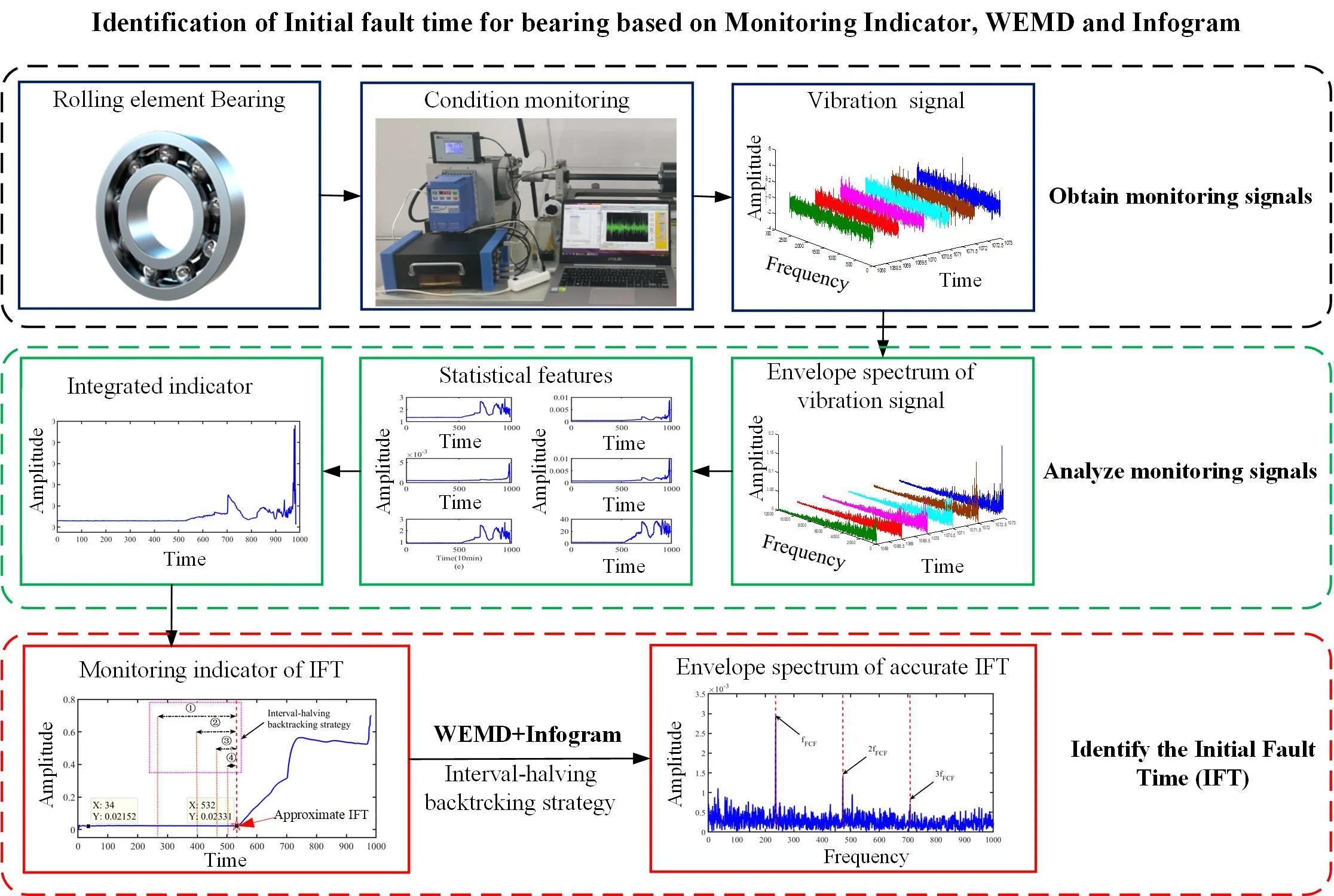
The flow chart of the proposed approach presented in Fig. 1 consists of the construction of the integrated indicator with the summation of multiple standardized features, the IFT identification based on the integrated indicator and envelope analysis with proposed WEMD and Infogram.
3.1. Construction of integrated indicator
All features of envelope spectrum can represent performance degradation of bearing, but their robustness is different. Meanwhile, their preferences are different to reflect the performance condition of bearing. The amplitude of every feature is different in the order of magnitudes. Therefore, the features with stably strong robustness should be selected to construct the integrated indicator, and these selected features should be standardized firstly to construct the integrated indicator. The integrated indicator can be obtained by the summation of multiple standardized features. The calculation of the integrated indicator contains three procedures.
Step 1. Selection of the features with stably strong robustness.
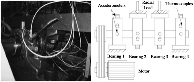
In order to select the features with stably strong robustness from the candidate features mentioned in Table 1, the tested data packet of bearings generated from the IMS Center of the University of Cincinnati is selected to analyze the robustness of the feature, which is also made public for the fault detection or diagnosis of bearings. The bearing test platform is shown in Fig. 2. Four Rexnord ZA-2115 double-row bearings were installed to support the shaft in the test platform, and its parameters are shown in Table 2. In order to fastly obtain the run-to-failure monitoring data similar to the real performance degradation of bearings, the shaft speed was kept at 2000 rpm (33.3 Hz) by an AC motor via a friction belt, and a radial load of 6000 lbs was put onto the shaft with a spring mechanism for reducing the service life in experiment. The tested data packet contains six run-to-failure datasets from three cases and is shown in Table 3. And test case will not end until one of the four bearings reached the complete failure in every case. Meanwhile, the complete failure time is older than the designed life time of bearings in every case. Every acquired vibration signal contains 20,480 points, which was collected by a data acquisition card (NI DAQ Card 6062E) every 10 min at a 20 kHz sampling rate. Two accelerometers were installed on the bearing housing of each bearing in case 1, which were placed vertically and horizontally, respectively. One accelerometer was only installed on the bearing housing of each bearing in case 2 and 3. The fault occurred in two of the bearings in case 1. The fault occurred in one of the bearings in case 2 and 3.
Fig. 1Flow chart of proposed approaches
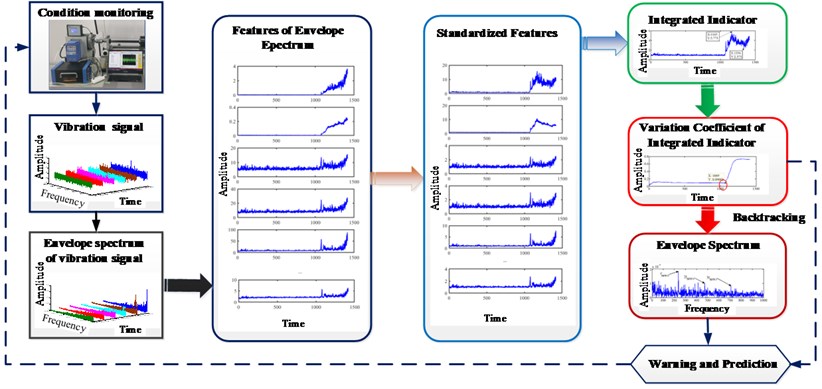
Fig. 2Test platform of bearings
The robustness of candidate features mentioned in Table 1 is calculated by Eq. (4) as shown in Table 4. From Table 4, the robustness of these features is not always beyond 0.9. Therefore, the Shape factor, Standard deviation, Average, RMS, Skewness and Variation Coefficient are selected to construct the integrated indicator.
Table 2Parameters of Rexnord ZA-2115 Double Row Bearing
Parameters | Ball number | Ball diameter | Pitch diameter | Contact angle |
Value | 16 | 8.4 | 71.5 | 15.17 |
Unit | / | mm | mm | ° |
Table 3Datasets from The IMS Center
Bearing of fault | Channel | Case | Defect type | Fault feature frequency | Number of sampling point |
3 | Ch 5 | 1 | Inner race | 296.9 Hz | 2156 |
3 | Ch 6 | 1 | Inner race | 296.9 Hz | 2156 |
4 | Ch 7 | 1 | Rolling element | 139.9 Hz | 2156 |
4 | Ch 8 | 1 | Rolling element | 139.9 Hz | 2156 |
1 | Ch 1 | 2 | Outer race | 236.4 Hz | 984 |
3 | Ch 3 | 3 | Outer race | 236.4 Hz | 6324 |
Table 4Robustness of features based on datasets from IMS Center
Datasets | Case1-Ch 5 | Case1-Ch 6 | Case1-Ch 7 | Case1-Ch 8 | Case2-Ch 1 | Case3-Ch 3 |
Clearance factor | 0.942 | 0.877 | 0.946 | 0.944 | 0.933 | 0.864 |
Crest factor | 0.942 | 0.888 | 0.948 | 0.946 | 0.939 | 0.865 |
Impulse factor | 0.942 | 0.877 | 0.946 | 0.944 | 0.934 | 0.864 |
Shape factor | 0.997 | 0.998 | 0.995 | 0.996 | 0.992 | 0.998 |
Standard deviation | 0.984 | 0.988 | 0.985 | 0.986 | 0.979 | 0.985 |
Average | 0.989 | 0.993 | 0.991 | 0.991 | 0.987 | 0.989 |
RMS | 0.988 | 0.992 | 0.989 | 0.990 | 0.983 | 0.988 |
Peak | 0.943 | 0.876 | 0.946 | 0.943 | 0.930 | 0.857 |
Skewness | 0.94 | 0.922 | 0.938 | 0.926 | 0.961 | 0.900 |
Kurtosis | 0.869 | 0.822 | 0.871 | 0.861 | 0.917 | 0.760 |
Variation Coefficient | 0.992 | 0.992 | 0.99 | 0.99 | 0.987 | 0.993 |
Step 2. Every feature is standardized in real time by Eq. (5):
where are the mean of every feature in real time, which is calculated based on the sampling data from the first to the current time.
Step 3. The integrated indicator is constructed by the summation of the multiple standardized features, which is calculated in real time by Eq. (6):
Step 4. Calculation of variation coefficient of the integrated indicator.
The variation coefficient of the integrated indicator can reflect the variation of the integrated indictor, which can be obtained by variation coefficient as Eq. (7):
where and is the standard deviation and mean of the integrated indicator in real time. They will be updated by the obtained integrated indicator from first to current sampling time.
Aiming at avoiding the is infinity, the current mean will be replaced with the previous mean when the calculated current mean is equal to 0 in practice.
3.2. Identification of IFT with approximate to fine strategy
Stage 1: Estimation of the approximate IFT. The approximate IFT can be obtained by the minimum before the early stage of the continuous increase in the variation coefficient of the integrated indicator. The approximate IFT indicates that a fault has been generated in bearing for warning and further reducing the detection range of the accurate IFT.
Stage 2: Identification of the accurate IFT. The accurate IFT can be acquired by the interval-halving backtracking strategy with envelope spectrum based on the proposed WEMD and Infogram. Firstly, the fault is detected by the envelope spectrum. Then, the fault is checked by the narrow-band envelope spectrum based on the proposed WEMD and Infogram when the FCF and its harmonics cannot be clearly seen in the envelope spectrum. Finally, the interval-halving backtracking process will end until the FCF and its harmonics cannot be clearly found in the narrow-band envelope spectrum. The interval-halving backtracking strategy was described by Meng et al. [11]. The WEMD will be detailed in the next part.
3.3. Identification of IFT with approximate to fine strategy
Due to the existence of over-decomposition or inadequate decomposition in EMD algorithm [34], the IMFs should be processed or selected for an ideal effect. There is a cyclostationary impact behavior in the vibration signal of fault bearing [38]. Because the strength of the impact component in the IMFs can be measured by the kurtosis, the correlation of the raw signal and the IMFs can be represented with the correlation coefficient. Hereafter the sensitivity of IMFs that contains the fault signature can be reflected by the value of the kurtosis and the correlation coefficient [39]. The signal can be reconstructed to enhance fault signature by the objective weight of IMFs and themselves. The improved EMD is named as the Weighted EMD (WEMD), which contains four procedures.
Step 1. Any signal is decomposed into individual components by EMD.
Step 2. The kurtosis and the correlation coefficient about each of IMFs are calculated.
Step 3. The weight of each of IMFs is obtained with Eq. (8):
Step 4. The highlighted fault signal is constructed with Eq. (9):
4. Simulation results and comparisons
The performance of the proposed WEMD method will be validated by the simulation signal. About 90 % of bearing failure results from defects in the inner or outer race [40]. The simulation signal of bearing with a defect can be constructed by Eqs. (10) [20, 36, 41]:
where is the possible amplitude of impulse response, is decay coefficient, is the resonant frequency, is the harmonic interference signal including harmonic signals, is Gaussian white noise, and are the amplitude and the angular frequency of the harmonic signal, respectively.
These parameters of the simulation signal are shown in Table 5. Furthermore, the simulation signal without white noise is shown in Fig. 3.
Table 5Parameters of the simulation signal
Parameters | SNR | ||||||
Value | [2.8 3.3] | 100 | 1300 Hz | 2 | 1.3/1.1 | 23 Hz/53 Hz | [–9 9] dB |
Fig. 3Simulation signal without white noise
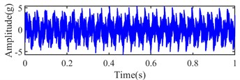
a) Signal in time domain
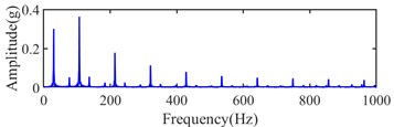
b) Envelope spectrum
The kurtosis is an indicator that reflects the strength of the impulse component in a signal [39]. The dispersion of signal intensity distribution is dominated by white noise except for the impulse component in a signal [42], and it can be measured with variance . In order to measure the SNR of the diagnosis signal, and considering that the impulse component in vibration signal of fault bearing should be concerned, the kurtosis and variance are used to represent the levels of signal and noise in SNR, respectively. The SNR can be replaced and measured by the Kurtosis-to-Variance Ratio (KVR) as Eq. (11):
The simulation signal with white noise at different SNR and its envelope spectrum are shown in Fig. 4. Their kurtosis, variance and KVR are shown in Table 6. The trend of the KVR is almost same as the SNR except for no noise from Table 6. The SNR is ineffective at no noise, and it is not existed for no noise in practice. Hence, the KVR can represent the SNR. Besides, the amplitude of the simulation signal at different SNR is enlarged as the noise increases, which causes an increase in kurtosis, but the increase in kurtosis is less than the change in variance since the increase of noise.
Fig. 4Simulation signal with white noise at different SNR
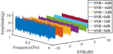
a) Signal in time domain
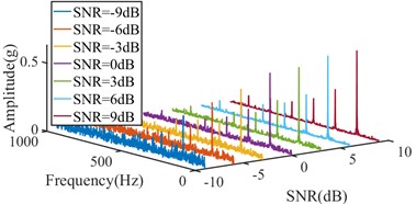
b) Envelope spectrum
Table 6Kurtosis, variance and sharpness of simulation signal with white noise at different SNR
SNR | –9 dB | –6 dB | –3 dB | 0 dB | 3 dB | 6 dB | 9 dB | No noise |
Kurtosis | 2.9131 | 2.8236 | 2.6452 | 2.4109 | 2.2666 | 2.1081 | 2.0353 | 1.933 |
Variance | 10.4974 | 6.2772 | 4.3866 | 3.4648 | 2.9768 | 2.7415 | 2.5987 | 2.4771 |
KVR | 0.2775 | 0.4498 | 0.603 | 0.6958 | 0.7617 | 0.769 | 0.7832 | 0.7803 |
In order to validate the effectiveness of the proposed WEMD, the simulation signal with –9 dB white noise is processed by different signal processing methods, and the simulation signal with –9 dB white noise is shown in Fig. 5. The simulation signal is reconstructed by the components of the maximum kurtosis and correlation coefficient with EMD and EEMD, and it is processed by WEMD. And beyond that, the unprocessed signal and the processed signal are filtered at the bandwidth and center frequency selected by Infogram. Their fitting density distributions, kurtosis, variance and KVR are shown in Fig. 6 and Table 7, respectively.
Fig. 5Simulation signal with -9 dB white noise
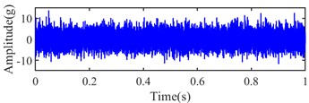
a) Signal in time domain
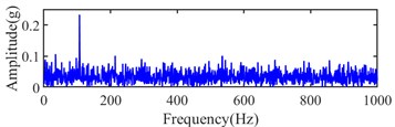
b) Envelope spectrum
From Table 7, the maximum KVR and minimum variance can be obtained by WEMD with Infogram. The largest KVR and smallest variance can also be obtained by WEMD among EMD, EEMD and WEMD. The largest kurtosis value of the signal can be obtained by the combined method of the EMD and EEMD with Infogram, but a strong noise is still present in the selected frequency band. Hence, their KVR is smaller than the WEMD with Infogram method. Based on these reasons, the proposed WEMD has an obvious advantage in denoising and enhancing fault signature. A better effect of the noise reduction and enhanced fault can be obtained by the combined signal processing method of WEMD and Infogram.
Fig. 6Fitting density distributions of the simulation signal with different processing methods
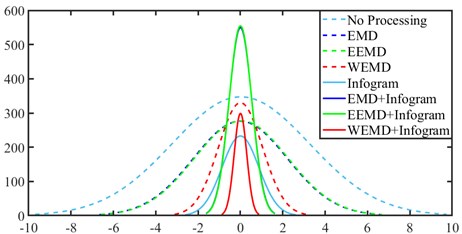
Table 7Kurtosis, variance and sharpness of simulation signal by different processing methods
Methods | No Processing | EMD | EEMD | WEMD | Infogram | EMD +Infogram | EEMD +Infogram | WEMD +Infogram |
Kurtosis | 3.0342 | 2.0071 | 2.638 | 2.9028 | 2.1173 | 6.504 | 6.6329 | 2.6143 |
Variance | 10.5337 | 4.5965 | 4.8987 | 0.9853 | 0.7565 | 0.294 | 0.2883 | 0.0876 |
KVR | 0.2881 | 0.4367 | 0.4232 | 3.01 | 2.7989 | 22.1246 | 23.0064 | 29.8391 |
5. Experimental results and analysis
The vibration data packet from the IMS Center mentioned in Section 3.1 has been applied multiple times for the experimental case study in [8-11, 14, 15, 35, 43]. The data packet contains three common fault types of bearings: outer race, inner race and rolling element. Meanwhile, all complete failures occurred after exceeding designed life time of bearings which is more than 100 million revolutions. Therefore, the run to failure data packet of bearing is also used to validate the proposed approach.
The datasets of bearing 3 in channel 5 of case 1, bearing 1 in channel 1 of case 2 and bearing 3 in channel 3 of case 3 mentioned in Table 3 are be analyzed detailly, and their run to failure vibration signals are shown in Fig. 7. From Fig. 7, the initial fault may be generated at about 1800th, 700th and 6100th sampling points in the three collected datasets.
5.1. Case 1
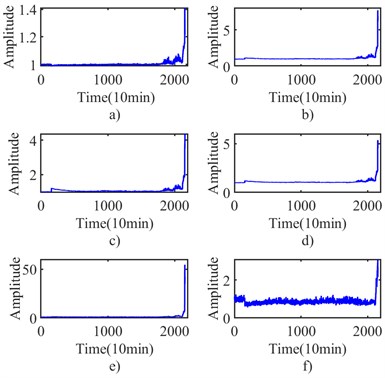
The experiment dataset of bearing 3 in Ch 5 of Case 1 is processed with the proposed method mentioned in Section 3. Initially, the collected signals are processed with envelope spectrum, and six selected indexes are obtained by the formulas mentioned in Table 1, and they are shown in Fig. 8. Next, the six indexes are standardized by Eq. (5) and shown in Fig. 9. The integrated indicator is obtained by Eq. (6) and shown in Fig. 10. The variation coefficient of the integrated indicator is obtained by Eq. (7) and shown in Fig. 11.
Fig. 7Vibration signals from IMS: a) case 1-Ch 5, b) case 2-Ch 1, c) case-Ch 3
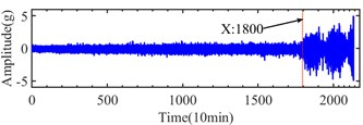
a)
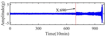
b)
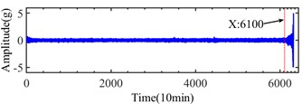
c)
Fig. 8Indexes of case 1: a) shape factor, b) standard deviation, c) average, d) RMS, e) variation coefficient, f) skewness
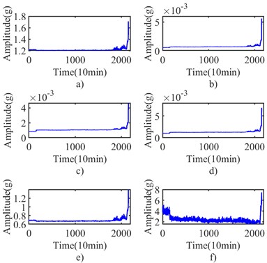
Fig. 9Standardized indexes of case 1: a) shape factor, b) standard deviation, c) average, d) RMS, e) variation coefficient, f) skewness
From Fig. 11, the approximate IFT can be estimated at the 1832th sampling point by the minimum before the early stage of the continuous increase in the curve of the variation coefficient of the integrated indicator. The Infogram of the 1832th sampling point is shown in Fig. 12. The bandwidth and center frequency of the Squared Envelope (SE), Squared Envelope Spectrum (SES) and average Infogram are identified as (10240 5120) Hz, (320, 9120) Hz and (10240, 5120) Hz, respectively. The fault characteristic frequency and its harmonics cannot be found in narrow-band envelope spectrum based on them. The optimal bandwidth should be selected within 3 and 6 times of fault characteristic frequency in the Shannon theorem. The optimal bandwidth is redressed as 1280 Hz at 5120 Hz and 9120 Hz center frequency, and its fault characteristic frequency and harmonics of fault characteristic frequency can be seen in envelope spectrum at (1280, 5120) Hz as shown in Fig. 13.
Fig. 10Integrated indicator of case 1
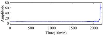
Fig. 11Variation coefficient of integrated indicator in case 1
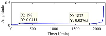
Fig. 12Infogram of the 1832th sampling point
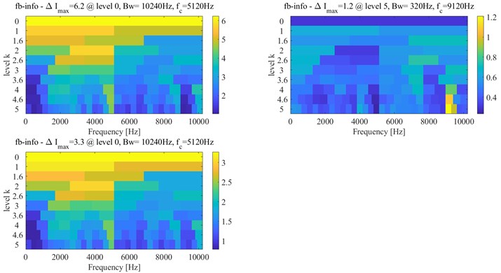
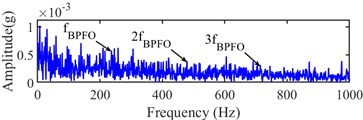
Fig. 13Narrow-band envelope spectrum of the 1832th sampling point
a) (1280, 5120) Hz
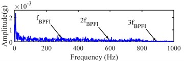
b) (1280, 9120) Hz
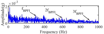
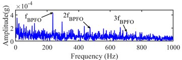
Meanwhile, the sampling point of the interval between 198th and 1832th sampling point are detected by interval-halving backtracking strategy with envelope spectrum based on WEMD and Infogram. However, the fault characteristic frequency and its harmonics cannot be seen in the envelope spectrum at the detected interval between 198th and 1831th sampling point. The bandwidth and center frequency of the SE, SES and average Infogram of 1831th sampling point are the same as the 1832th sampling point, and the envelope spectrums are shown in Fig. 14, and the fault characteristic frequency and its harmonics cannot be found at their envelope spectrum. Hence, the 1832th sampling point is finally recognized as the accurate IFT by the interval-halving backtracking strategy.
Table 8IFT of other datasets in case 1
Bearing of fault | Channel | IFT |
Bearing 3 | Ch 6 | 1840th |
Bearing 4 | Ch 7 | 1440th |
Bearing 4 | Ch 8 | 1441th |
Besides, the other three collected datasets in case 1 are also analyzed by using the same way. Their results are shown in Table 8.
Fig. 14Narrow-band envelope spectrum of the 1831th sampling point
a) (1280, 5120) Hz
b) (1280, 9120) Hz
5.2. Case 2
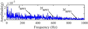
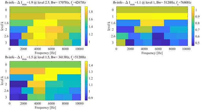
The experiment dataset of bearing 1 in Ch 1 of case 2 is analyzed by using the same method as case 1. The integrated indicator and its variation coefficients are obtained based on six selected indexes, which are shown in Fig. 15 and Fig. 16, respectively. According to Fig. 16, the approximate IFT can be estimated at the 532th sampling point, and the optimal bandwidth and center frequency are estimated as (1707, 4267) Hz, (5120, 7680) Hz and (3413 5120) Hz based on the SE, SES and average Infogram, which is shown in Fig. 17, respectively. However, the fault characteristic frequency and its harmonics can be found in their narrow-band envelope spectrum. Because of the optimal bandwidth limitation of the Shannon theorem, the bandwidth is reset as 1280 Hz. The fault characteristic frequency and its harmonics can be found at narrow-band envelope spectrum of (1280, 7680) Hz, which is shown in Fig. 18.
Fig. 15Integrated indicator of case 2
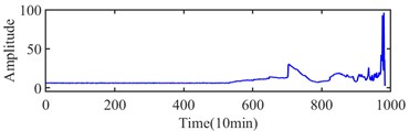
Fig. 16Variation coefficients of integrated indicator in case 2
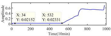
Fig. 17Infogram of the 532th sampling point
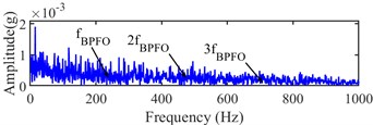
The further detected interval is determined at the interval between 34th and 532th sampling points. The accurate IFT is further found at the 524th sampling point by the interval-halving backtracking strategy. The Infogram of the 524th sampling point is shown in Fig. 19. The (1280 5760) Hz and (5120, 7680) Hz are identified as the optimal bandwidth and center frequency by Infogram, respectively. The optimal bandwidth should be limited at between 3 and 6 times of fault characteristic frequency in the Shannon theorem. The optimal bandwidth of 1280 Hz is used for envelop analysis, the envelope spectrums of the 524th sampling point are shown in Fig. 20.
Fig. 18Narrow-band envelope spectrum of the 532th sampling point
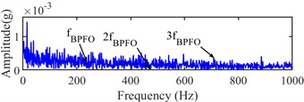
a) [1280, 4267] Hz
b) [1280, 5120] Hz
c) [1280, 7680] Hz
Fig. 19Infogram of the 524th sampling point
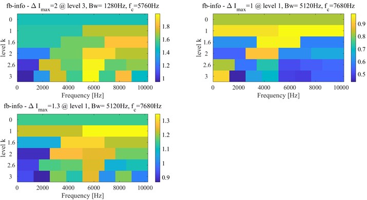
Fig. 20Narrow-band envelope spectrum of the 524th sampling point
a) (1280, 5760) Hz
b) (1280, 7680) Hz
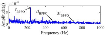
Fig. 21Narrow-band envelope spectrum of the 523th sampling point
a) (1280, 5760) Hz
b) (1280, 7680) Hz
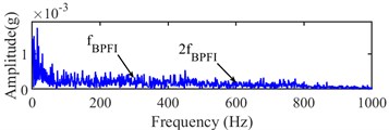
The fault characteristic frequency and its 2x and 3x harmonic can be found at (1280, 7680) Hz from Fig. 20(b). The 523th sampling point is analyzed as the same as the 524th sampling point. Its Infogram is the same as the Infogram of the 524th sampling point. From Fig. 21 of narrow-band envelope spectrums at (1280, 5120) Hz and (1280, 7680) Hz of the 523th sampling point, the fault characteristic frequency is only found, but its harmonics cannot be found. Hence, the 524th sampling point can be regarded as the accurate IFT.
5.3. Case 3
The experiment dataset of bearing 3 in Ch 3 of case 3 is analyzed by the same method as case 1 and 2. The integrated indicator and its variation coefficient are shown in Figs. 22 and 23, respectively.
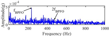
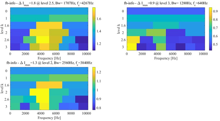
According to Fig. 23, the approximate IFT can be estimated at the 5965th sampling point, and the further detected interval is determined at between 274th and 5965th sampling points. The Infogram of the 5965th sampling point is shown in Fig. 24, and the (1707 4267) Hz, (1280, 640) Hz and (2560, 3840) Hz are identified as the optimal bandwidth and center frequency by the SE, SES and average Infogram, respectively. The optimal bandwidth is changed to 1280 Hz, and the bandwidth at the center frequency of 640 Hz is reset as 1200 Hz. The fault characteristic frequency and its 3x harmonics can be found at envelope spectrum based on (1280, 3840) Hz as shown in Fig. 25(c).
Fig. 22Integrated indicator of case 3
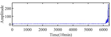
Fig. 23Variation coefficients of integrated indicator in case 3
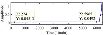
Fig. 24Infogram of the 5965th sampling point
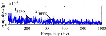
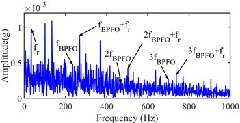
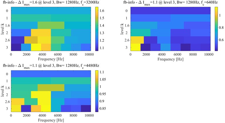
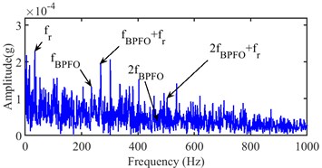
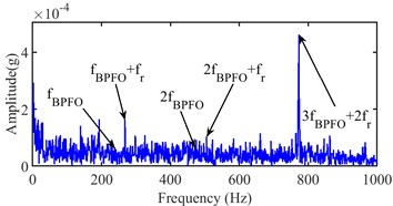
The accurate IFT is further found at the 5900th sampling point by the interval-halving backtracking strategy. The Infogram of the 5900th sampling point is shown in Fig. 26, the optimal bandwidth and center frequency (1280, 3200) Hz, (1280, 640) Hz and (1280 4480) Hz are recognized with the SE, SES and average Infogram, respectively. The bandwidth is reset as 1200 Hz of the center frequency at 640 Hz to obtain the narrow-band envelope spectrum. And their narrow-band envelope spectrums are shown in Fig. 27. The BPFO can be obviously seen in the (1280, 3200) Hz from Fig. 27(a), the BPFO and 2x harmonic of BPFO is seen in the (1200, 640) Hz from Fig. 27(b) and its 2x and 3x harmonic of BPFO cannot be seen in the (1280, 4480) Hz from Fig. 27(c). Besides, the BPFO and its harmonics with rotational frequency are also found in Fig. 27.
Fig. 25Narrow-band envelope spectrum of the 5965th sampling point
a) (1707, 4267) Hz
b) (1200, 640) Hz
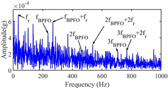
c) (1280, 3840) Hz
Fig. 26Infogram of the 5900th sampling point
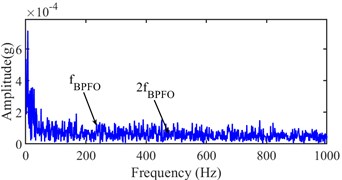
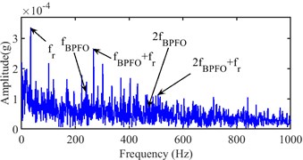
Meanwhile, the 5899th sampling point is also analyzed by the same method as the 5900th sampling point. Its Infogram is shown in Fig. 28, and the optimal bandwidth and center frequency (1707, 4267) Hz and (1280, 640) Hz can be obtained by the Infogram. The optimal bandwidth and center frequency are redressed as (1280, 4267) Hz and (1200, 640) Hz based on Shannon theorem and envelope spectrum, and their narrow-band envelope spectrums are shown in Fig. 29. The BPFO is only obviously seen in Fig. 29 a). Although the BPFO and its harmonics with rotational frequency can be found in Fig. 29, its harmonics cannot be found in Fig. 29. The existence of fault is not determined by its envelope spectrum. Hence, the accurate IFT is considered at the 5900th sampling point.
Fig. 27Narrow-band envelope spectrum of the 5900th sampling point
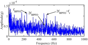
a) (1280 3200) Hz
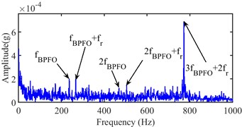
b) (1200 640) Hz
c) (1280 4480) Hz
Fig. 28Infogram of the 5899th sampling point
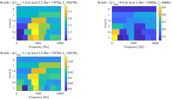
Fig. 29Narrow-band envelope spectrum of the 5899th sampling point
a) (1280 4267) Hz
b) (1200 640) Hz
6. Comparisons and discussions
Aiming at verifying the accuracy of the identified IFT of bearings, the results are compared with other previous investigations [8-11, 14, 15, 44] and these identified methods with the fault diagnosis techniques are described in Table 9. And these identified initial fault results have been detailed in Tables 10, 11 and 12 based on cases 1, 2 and 3, respectively. There are few identified results of case 1 since the monitoring of inner race faults is more difficult and its investigation is less [11, 45]. The vibration data of case 3 is less used in previous articles since the data was updated behind cases 1 and 2 [11].
Table 9Description of identified methods for initial fault time
Methods | Description of method |
Method 1 [8] | Calculate the proposed threshold ( and are the mean and standard deviation of EHNR) based on EHNR by FEEMD. |
Method 2 [8] | Calculate the proposed threshold ( and are the mean and standard deviation of EEACF) based on EEACF. |
Method 3 [9] | Coarse-to-fine strategy based on envelope spectrum by using VMD and MOMEDA. |
Method 4 [10] | Backtracking strategy based on envelope spectrum by using improved VMD and Infogram. |
Method 5 [11] | Backtracking strategy based on envelope spectrum by using EMD-Fast ICA. |
Method 6 [14] | Detect the incipient fault of bearing by IVMD conjoined EMD. |
Method 7 [15] | An almost the same kurtosis values in multiple components based on improved TQWT. |
Method 8 [44] | A scale independent flexible bearing health monitoring index based on time frequency manifold energy & entropy. |
Proposed method | Approximate to accurate strategy based on envelope spectrum by using monitoring indicator and WEMD with Infogram. |
Table 10Comparisons of the initial fault point in case 1
Methods | Method 1 [8] | Method 2 [8] | Method 5 [11] | Method 7 [15] | The proposed method (approximate) | The proposed method (accurate) |
IFTs | 2120th | Ineffective | 1990th | 1980th | 1832th | 1832th |
Table 11Comparisons of the initial fault point in case 2
Methods | Method 1 [8] | Method 2 [8] | Method 3 [9] | Method 4 [10] | Method 5 [11] | Method 6 [14] | Method 7 [15] | Method 8 [47] | The proposed method (approximate) | The proposed method (accurate) |
IFTs | 535th | 533th | 533th | 531th | 533th | 531th | 532th | 533th | 532th | 524th |
Table 12Comparisons of the initial fault point in case 3
Methods | Method 1 [8] | Method 2 [8] | Method 7 [15] | The proposed method (approximate) | The proposed method (accurate) |
IFTs | 6162th | 6072th | 6071th | 5965th | 5900th |
According to the comparisons of the estimated approximate IFT with the results of other methods, the results show that the identification method of the approximate IFT is almost as accurate as other methods, or even more accurate. Meanwhile, the variation coefficient of the integrated indicator can be obtained timely based on the monitoring data from first to current monitoring time. The IFT can be monitored by the minimum before the early stage of continuous increase in variation coefficient of the integrated indicator in practice.
In addition, an earlier IFT can be found rapidly by interval-halving backtracking strategy with envelope analysis based on the proposed WEMD and Infogram. The earlier IFT has better accuracy than the results of other methods and the approximate IFT. The more accurate IFT can help to improve the accuracy of RUL prediction further. Meanwhile, the simulation results and the earlier IFT show that the combination of the WEMD and Infogram has a good effect on denoising or enhancement of the fault component in the vibration signal.
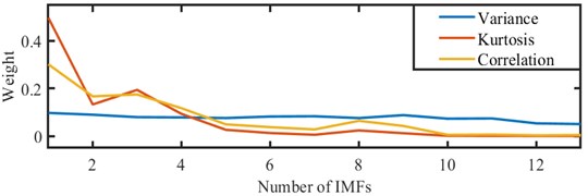
Meanwhile, the weight of every IMFs in variance, kurtosis and correlation coefficient are analyzed in EMD based on the simulation signal, which is shown in Fig. 30. From Fig. 30, there is a similar and obvious change in the weight of kurtosis and correlation coefficient, but there's almost no weight difference in variance. The weight of kurtosis and correlation coefficient is greater than the weight of variance in some IMFs, and other IMFs is smaller. The KVR of the IMFs with large KVR become larger and the KVR of IMFs with small KVR become smaller by the weight operator in WEMD. Therefore, the WEMD can improve the KVR of signal, which has a better effect than EMD and EEMD on denoising or enhancing the fault component.
Fig. 30Weight of every IMFs in variance, kurtosis and correlation coefficient
There is a difference in the recognized IFT of bearing 3 based on Ch 5 and Ch 6 and the bearing 4 based on Ch 7 and Ch 8 in case 1. The difference of the recognized IFT of the bearing 3 based on two channels may be caused by two accelerometer positions and the rotation of inner race. Two accelerometer positions have different sensitivity to the generated location of the fault. And the different sensitivity may be verified at bearing 4 based on Ch 7 and Ch 8 in case 1, and there is also a slight difference at bearing 4 based on two-channel signals.
There is an irregularity in the integrated indicator curve in Figs. 10, 15 and 22. The irregularity may be on account of bearing manufacturing errors, unstable rotor speed, friction and poor lubrication etc. And there is some larger fluctuation at the unhealthy condition in Figs. 10, 15 and 22, which may be due to the abrasive particles dropping into the defect, the edge of the defect being smoothed or the impact behavior from the defect.
There is a short rise in the early stage of the variation coefficient of the integrated indicator in Figs. 11, 16 and 23, which may be a running-in phase as described in [43]. The running-in phase is the earlier stage of perfectly healthy conditions of bearings, moreover which is healthy. There may be an uneven distribution of the grease or some degrees of surface waviness and surface roughness in a new bearing. The phase usually ends very quickly with normal running after some wear [46]. Then, the performance of bearings starts to weaken slowly with the repeated cyclic contact of rolling elements and inner or outer race. And the variation of bearings performance is slower and slower until a fault occurred. The performance of bearings will generally become worse and worse after the existence of a fault, and the variation of bearings performance is faster and faster in general. When the unhealthy condition reaches a certain level, the severity is almost constant or diminishing. Hence, the variation coefficient of the integrated indicator of the bearings performance degradation features can represent the variation of the performance for monitoring the IFT of bearings. However, a quite accurate IFT has been found before the minimum before the early stage of the continuous increase in the variation coefficient of the integrated indicator. However, the initial fault is generally a micro-crack in the beginning because repeated cycles of contact result in the accumulation of plastic strain [43]. The fault is so weak that it cannot be highlighted in the performance degradation indicator of bearing. Therefore, the identification mechanism from the approximate to the more accurate IFT is not in conflict with the fact.
7. Conclusions
An approximate to fine identified method of the IFT of bearing is proposed for monitoring the IFT and improving the accuracy of RUL prediction in the article. Firstly, an approximate IFT can be obtained by the minimum before the early stage of the continuous increase of the constructed variation coefficient of the integrated indicator. Whereafter, a more accurate IFT can be obtained by interval-halving backtracking strategy based on WEMD, Infogram and envelope analysis. Some conclusions could be given as follows.
1) The variation coefficient of the integrated indicator can be used to monitor the health condition of bearings, and the minimum before the early stage of the continuous increase of the constructed variation coefficient of the integrated indicator can be used to obtain the approximate IFT.
2) The more accurate IFT can be obtained rapidly by the interval-halving backtracking strategy based on WEMD, Infogram and envelope analysis.
3) The combined method of WEMD and Infogram can be applied for denoising or enhancing the fault component in vibration signal with fault.
References
-
Y. Lu, R. Xie, and S. Y. Liang, “Detection of weak fault using sparse empirical wavelet transform for cyclic fault,” The International Journal of Advanced Manufacturing Technology, Vol. 99, No. 5-8, pp. 1195–1201, Nov. 2018, https://doi.org/10.1007/s00170-018-2553-1
-
X. Ding, Q. He, and N. Luo, “A fusion feature and its improvement based on locality preserving projections for rolling element bearing fault classification,” Journal of Sound and Vibration, Vol. 335, pp. 367–383, Jan. 2015, https://doi.org/10.1016/j.jsv.2014.09.026
-
A. Rai and S. H. Upadhyay, “A review on signal processing techniques utilized in the fault diagnosis of rolling element bearings,” Tribology International, Vol. 96, pp. 289–306, Apr. 2016, https://doi.org/10.1016/j.triboint.2015.12.037
-
R. B. Randall, Vibration-based Condition Monitoring: Industrial, Aerospace and Automotive Applications. Hoboken, New Jersey, United Kingdom: John Wiley & Sons, 2011.
-
J. Lee, F. Wu, W. Zhao, M. Ghaffari, L. Liao, and D. Siegel, “Prognostics and health management design for rotary machinery systems-Reviews, methodology and applications,” Mechanical Systems and Signal Processing, Vol. 42, No. 1-2, pp. 314–334, Jan. 2014, https://doi.org/10.1016/j.ymssp.2013.06.004
-
Y. Lei, N. Li, L. Guo, N. Li, T. Yan, and J. Lin, “Machinery health prognostics: A systematic review from data acquisition to RUL prediction,” Mechanical Systems and Signal Processing, Vol. 104, pp. 799–834, May 2018, https://doi.org/10.1016/j.ymssp.2017.11.016
-
N. Li, Y. Lei, J. Lin, and S. X. Ding, “An improved exponential model for predicting remaining useful life of rolling element bearings,” IEEE Transactions on Industrial Electronics, Vol. 62, No. 12, pp. 7762–7773, Dec. 2015, https://doi.org/10.1109/tie.2015.2455055
-
A. Babiker, C. Yan, Q. Li, J. Meng, and L. Wu, “Initial fault time estimation of rolling element bearing by backtracking strategy, improved VMD and Infogram,” Journal of Mechanical Science and Technology, Vol. 35, No. 2, pp. 425–437, Feb. 2021, https://doi.org/10.1007/s12206-021-0101-7
-
Q. Li, C. Yan, W. Wang, A. Babiker, and L. Wu, “Health indicator construction based on MD-CUMSUM with multi-domain features selection for rolling element bearing fault diagnosis,” IEEE Access, Vol. 7, pp. 138528–138540, 2019, https://doi.org/10.1109/access.2019.2942371
-
J. Meng, C. Yan, G. Chen, Y. Liu, and L. Wu, “Health indicator of bearing constructed by RMS-CUMSUM and GRRMD-CUMSUM with multifeatures of envelope spectrum,” IEEE Transactions on Instrumentation and Measurement, Vol. 70, pp. 1–16, 2021, https://doi.org/10.1109/tim.2021.3054000
-
S. N. Chegini, M. J. H. Manjili, and A. Bagheri, “New fault diagnosis approaches for detecting the bearing slight degradation,” Meccanica, Vol. 55, No. 1, pp. 261–286, Jan. 2020, https://doi.org/10.1007/s11012-019-01116-x
-
I. M. Howard, “A review of rolling element bearing vibration detection, diagnosis and prognosis,” DSTO Aeronautical and Maritime Research Laboratory, 1994.
-
Y. Wang, Y. Peng, Y. Zi, X. Jin, and K.-L. Tsui, “A two-stage data-driven-based prognostic approach for bearing degradation problem,” IEEE Transactions on Industrial Informatics, Vol. 12, No. 3, pp. 924–932, Jun. 2016, https://doi.org/10.1109/tii.2016.2535368
-
F. Jiang, Z. Zhu, and W. Li, “An improved VMD with empirical mode decomposition and its application in incipient fault detection of rolling bearing,” IEEE Access, Vol. 6, pp. 44483–44493, 2018, https://doi.org/10.1109/access.2018.2851374
-
P. Ma, H. Zhang, W. Fan, and C. Wang, “Early fault diagnosis of bearing based on frequency band extraction and improved tunable Q-factor wavelet transform,” Measurement, Vol. 137, pp. 189–202, Apr. 2019, https://doi.org/10.1016/j.measurement.2019.01.036
-
H. Cao, L. Niu, S. Xi, and X. Chen, “Mechanical model development of rolling bearing-rotor systems: A review,” Mechanical Systems and Signal Processing, Vol. 102, pp. 37–58, Mar. 2018, https://doi.org/10.1016/j.ymssp.2017.09.023
-
N. E. Huang et al., “The empirical mode decomposition and the Hilbert spectrum for nonlinear and non-stationary time series analysis,” Proceedings of the Royal Society of London. Series A: Mathematical, Physical and Engineering Sciences, Vol. 454, No. 1971, pp. 903–995, Mar. 1998, https://doi.org/10.1098/rspa.1998.0193
-
T. Zan, Z. Pang, M. Wang, and X. Gao, “Research on early fault diagnosis of rolling bearing based on VMD,” in 2018 6th International Conference on Mechanical, Automotive and Materials Engineering (CMAME), pp. 41–5, Aug. 2018, https://doi.org/10.1109/cmame.2018.8592450
-
X. An, H. Zeng, W. Yang, and X. An, “Fault diagnosis of a wind turbine rolling bearing using adaptive local iterative filtering and singular value decomposition,” Transactions of the Institute of Measurement and Control, Vol. 39, No. 11, pp. 1643–1648, Nov. 2017, https://doi.org/10.1177/0142331216644041
-
J. Luo and S. Zhang, “Rolling bearing incipient fault detection based on a multi-resolution singular value decomposition,” Applied Sciences, Vol. 9, No. 20, p. 4465, Oct. 2019, https://doi.org/10.3390/app9204465
-
L. Zhang, Z. Wang, and L. Quan, “Research on weak fault extraction method for alleviating the mode mixing of LMD,” Entropy, Vol. 20, No. 5, p. 387, May 2018, https://doi.org/10.3390/e20050387
-
A. Tabrizi, L. Garibaldi, A. Fasana, and S. Marchesiello, “Early damage detection of roller bearings using wavelet packet decomposition, ensemble empirical mode decomposition and support vector machine,” Meccanica, Vol. 50, No. 3, pp. 865–874, Mar. 2015, https://doi.org/10.1007/s11012-014-9968-z
-
Y. Li, X. Liang, M. Xu, and W. Huang, “Early fault feature extraction of rolling bearing based on ICD and tunable Q-factor wavelet transform,” Mechanical Systems and Signal Processing, Vol. 86, pp. 204–223, Mar. 2017, https://doi.org/10.1016/j.ymssp.2016.10.013
-
X. Yan, Y. Xu, D. She, and W. Zhang, “A bearing fault diagnosis method based on PAVME and MEDE,” Entropy, Vol. 23, No. 11, p. 1402, Oct. 2021, https://doi.org/10.3390/e23111402
-
G. Taguchi, S. Chowdhury, and Y. Wu, Taguchi’s Quality Engineering Handbook. Hoboken, New Jersey, United Kingdom: John Wiley and Sons, 2007.
-
J. Yu, “Bearing performance degradation assessment using locality preserving projections and Gaussian mixture models,” Mechanical Systems and Signal Processing, Vol. 25, No. 7, pp. 2573–2588, Oct. 2011, https://doi.org/10.1016/j.ymssp.2011.02.006
-
G. Jia, S. Yuan, and C. Tang, “Fault diagnosis of roller bearing based on PCA and multi-class support vector machine,” in Computer and Computing Technologies in Agriculture IV, pp. 198–205, 2011, https://doi.org/10.1007/978-3-642-18369-0_22
-
B. Wang, F. Wang, B. Dun, X. Chen, D. Yan, and H. Zhu, “Remaining life prediction of rolling bearing based on PCA and improved logistic regression model,” Journal of Vibroengineering, Vol. 18, No. 8, pp. 5192–5203, Dec. 2016, https://doi.org/10.21595/jve.2016.17449
-
X. Jiang, J. Wang, J. Shi, C. Shen, W. Huang, and Z. Zhu, “A coarse-to-fine decomposing strategy of VMD for extraction of weak repetitive transients in fault diagnosis of rotating machines,” Mechanical Systems and Signal Processing, Vol. 116, pp. 668–692, Feb. 2019, https://doi.org/10.1016/j.ymssp.2018.07.014
-
A. Soylemezoglu, S. Jagannathan, and C. Saygin, “Mahalanobis Taguchi System (MTS) as a prognostics tool for rolling element bearing failures,” Journal of Manufacturing Science and Engineering, Vol. 132, No. 5, Oct. 2010, https://doi.org/10.1115/1.4002545
-
D. Liparas, L. Angelis, and R. Feldt, “Applying the Mahalanobis-Taguchi strategy for software defect diagnosis,” Automated Software Engineering, Vol. 19, No. 2, pp. 141–165, Jun. 2012, https://doi.org/10.1007/s10515-011-0091-2
-
J. Chen, L. Cheng, H. Yu, and S. Hu, “Rolling bearing fault diagnosis and health assessment using EEMD and the adjustment Mahalanobis-Taguchi system,” International Journal of Systems Science, Vol. 49, No. 1, pp. 147–159, Jan. 2018, https://doi.org/10.1080/00207721.2017.1397804
-
P. Shakya, M. S. Kulkarni, and A. K. Darpe, “A novel methodology for online detection of bearing health status for naturally progressing defect,” Journal of Sound and Vibration, Vol. 333, No. 21, pp. 5614–5629, Oct. 2014, https://doi.org/10.1016/j.jsv.2014.04.058
-
Y. Lei, J. Lin, Z. He, and M. J. Zuo, “A review on empirical mode decomposition in fault diagnosis of rotating machinery,” Mechanical Systems and Signal Processing, Vol. 35, No. 1-2, pp. 108–126, Feb. 2013, https://doi.org/10.1016/j.ymssp.2012.09.015
-
Z. Wang, C. Lu, Z. Wang, H. Liu, and H. Fan, “Fault diagnosis and health assessment for bearings using the Mahalanobis-Taguchi system based on EMD-SVD,” Transactions of the Institute of Measurement and Control, Vol. 35, No. 6, pp. 798–807, Aug. 2013, https://doi.org/10.1177/0142331212472929
-
P. Borghesani, P. Pennacchi, and S. Chatterton, “The relationship between kurtosis – and envelope-based indexes for the diagnostic of rolling element bearings,” Mechanical Systems and Signal Processing, Vol. 43, No. 1-2, pp. 25–43, Feb. 2014, https://doi.org/10.1016/j.ymssp.2013.10.007
-
B. Zhang, L. Zhang, and J. Xu, “Degradation feature selection for remaining useful life prediction of rolling element bearings,” Quality and Reliability Engineering International, Vol. 32, No. 2, pp. 547–554, Mar. 2016, https://doi.org/10.1002/qre.1771
-
T. Gerber, N. Martin, and C. Mailhes, “Time-frequency tracking of spectral structures estimated by a data-driven method,” IEEE Transactions on Industrial Electronics, Vol. 62, No. 10, pp. 6616–6626, Oct. 2015, https://doi.org/10.1109/tie.2015.2458781
-
X. Zhang, Z. Liu, Q. Miao, and L. Wang, “An optimized time varying filtering based empirical mode decomposition method with grey wolf optimizer for machinery fault diagnosis,” Journal of Sound and Vibration, Vol. 418, pp. 55–78, Mar. 2018, https://doi.org/10.1016/j.jsv.2017.12.028
-
J. Sandy, “Monitoring and diagnostic for rolling element bearings,” Sound and Vibration, Vol. 6, pp. 16–22, 1988.
-
I. Attoui, B. Oudjani, N. Boutasseta, N. Fergani, M.-S. Bouakkaz, and A. Bouraiou, “Novel predictive features using a wrapper model for rolling bearing fault diagnosis based on vibration signal analysis,” The International Journal of Advanced Manufacturing Technology, Vol. 106, No. 7-8, pp. 3409–3435, Feb. 2020, https://doi.org/10.1007/s00170-019-04729-4
-
K. F. Al-Raheem, A. Roy, K. P. Ramachandran, D. K. Harrison, and S. Grainger, “Rolling element bearing faults diagnosis based on autocorrelation of optimized: wavelet de-noising technique,” The International Journal of Advanced Manufacturing Technology, Vol. 40, No. 3-4, pp. 393–402, Jan. 2009, https://doi.org/10.1007/s00170-007-1330-3
-
I. El-Thalji and E. Jantunen, “A descriptive model of wear evolution in rolling bearings,” Engineering Failure Analysis, Vol. 45, pp. 204–224, Oct. 2014, https://doi.org/10.1016/j.engfailanal.2014.06.004
-
K. Noman, Q. He, Z. Peng, and D. Wang, “A scale independent flexible bearing health monitoring index based on time frequency manifold energy and entropy,” Measurement Science and Technology, Vol. 31, No. 11, p. 114003, Nov. 2020, https://doi.org/10.1088/1361-6501/ab9412
-
J. R. Stack, T. G. Habetler, and R. G. Harley, “Fault-signature modeling and detection of inner-race bearing faults,” IEEE Transactions on Industry Applications, Vol. 42, No. 1, pp. 61–68, Jan. 2006, https://doi.org/10.1109/tia.2005.861365
-
N. K. Arakere and G. Subhash, “Work hardening response of M50-NiL case hardened bearing steel during shakedown in rolling contact fatigue,” Materials Science and Technology, Vol. 28, No. 1, pp. 34–38, Jan. 2012, https://doi.org/10.1179/1743284711y.0000000060
Cited by
About this article

This work was supported by the National Natural Science Foundation of China (Grant No. 51765034), the Science and Technology Projects of Gansu Province (Project No. 21JR7RA305), and the Key Laboratory of Cloud Computing of Gansu Province (Gansu Computing Center).
