Abstract
An innovative design of a solar natural vacuum desalination (SNVD) system is proposed and investigated. To obtain a vacuum pressure in a desalination chamber its height is considered as 9.5 m. The waste heat in the system is efficiently utilized for both brine and distilled water. Seawater is preheated by the produced warm water, then, it is heated again by the outlet rejected hot brine before it is charged into the evaporation chamber. In addition, inlet pure water to a flat-plate collector is preheated by the condensation latent heat of the evaporated vapor from the evaporation chamber. Later, the outlet hot water from the collector is used as a heat source to the evaporation process. An optimum design of the system components was provided under the actual weather conditions for the shortest day of the year. It was found that the collector area is required to be 23 m2 to produce 66.6 liter of distilled water during. A mathematical modeling of the system was provided to establish a transient simulation and investigate the hourly performance of the system. Based on the annual performance of the system, the system can produce 76.5 liter of distilled water daily that is corresponding to 3.5 liter per one quadratic meter of collector. The annual average specific productivity of the system is obtained as 1.44 liter per kWh of solar radiation. Moreover, the maximum annual production is estimated as 92.88 liter of distilled water per day. Accordingly, the evaporation ratio (ER) is dependent on the solar irradiation and the annual average is found 0.0175 (or 1.75 %) where the gain output ratio (GOR) was estimated as 0.97 on yearly average basis.
1. Introduction
It is well defined that world suffers from lack of potable fresh water, pollution of the ecology and environment, shortage of natural and fossil fuels and also steadily increasing energy prices. Nowadays, the availability of freshwater is one of the most major problems facing the world. Over a billion people do not have access to clean water today, according to estimates [1].
Distillation is the process by which the contaminants and impurities are effectively removed from impure water. Several techniques and methodologies are used to make saline water (brackish water) potable. For example, filtration, sterilization, precipitation, and chemical treatment are some processes used to remove macro (visible) impurities and heavy particles from impure and contaminated water.
Although there are several traditional desalination techniques, solar water desalination (SWD) techniques are suitable technique to convert saline and brackish water into fresh water. These techniques have received greater attention. Solar energy is considered as a plentiful and effortlessly available renewable energy [2].
Solar water desalination techniques are, in general, classified as direct and indirect techniques. In direct method, feed water (i.e., saline or sea water) is directly absorbed by the solar radiator. However, for indirect methods, solar thermal collectors and photovoltaic (PV) are used. solar thermal collectors absorb solar radiation and then transfer the heat to the saline water. PV panels are used to convert solar radiation into electricity which used to run the desalination plant. Multi-stage flash distillation (MSFD), multi-effect distillation (MED), vapor compression distillation (VC) and Freezing are the major indirect desalination types in which solar collectors are used. Reverse osmosis (RO) and Electro-dialysis are, also, the major indirect desalination types in which PV panels are used [2], [3]. MSFD and RO are now in use. These two approaches, which require large amounts of fundamental thermal and/or electrical energy to produce fresh water from saltwater or sea water, are in use in large-scale facilities generating millions of gallons of pure water. The humidification-dehumidification (HDH) method has been found to be a cost-effective and efficient technique of desalination [4]. MED is older than MSFD. However, MED lost its popularity because it suffered some operational problems and was limited to the maximum size of the units [5].
The choice between these desalination processes is based on technical, economic and political bases. For large-scale productions, MSFD is the most popular among the desalination processes [5].
Various studies related to barometric desalination have been developed throughout the previous decades [6]. Al-Kharabsheh and Goswami [7] investigated evaporation and condensation in vacuum circumstances. Water distillation at a lower temperature level consumes less thermal energy. Solar collectors can produce this heat. Bemporad [8] devised a method for simulating evaporation rates in evaporators. This model was used to determine the system's optimal operating conditions and parameters. Bemporad discovered that the production rate was mostly determined by the temperature of the saline water. As the temperature of saline water rises, the difference in temperature between the two sides increases as well (which is the driving force). The optimal operating conditions, according to Bemporad, are 0.08 m water depth in the evaporator and 0.1 kg/h brine extraction rate. The system’s output fresh water rate was reported as 0.1739 kg/h. After that, an experimental system was built up with a 0.2 m2 evaporator area, heated by an electric heater to imitate the impact of solar panel heating [7], and the experimental production rate was around 5 %-10 % lower than that anticipated by the simulated process.
Midilli and Ayhan [9] conducted research that ran concurrently with Bemporad's research. Both researches had a similar design and principles. However, the vapor was driven from the evaporator to the condenser by a fan. A thermodynamic study of the process under free and forced convection was provided by Midilli and Ayhan. The model was created with solar energy in mind. Midilli and Ayhan [10] built an experimental system based on the design provided by the theoretical model. Free and forced mass convection were used in the studies. They observed that the production rate is lower than the theoretical model predicts. The theoretical and practical experiments yielded maximal freshwater production rates of 9.79 and 3.96 kg/h, respectively [10]. The experimental set-up used almost three times the amount of power predicted by the theoretical study. These discrepancies, according to Midilli and Ayhan, are due to heat and pressure losses in the connections. Jitsuno and Hamabe [11], recently, performed tests on a system that used a simulated NVD model. They built an experimental system; this system was evacuated by a vacuum pump. The rate of freshwater generation was reported to be 0.42 kg/h/m2 of evaporator area.
Reali et al [12] propose another barometric desalination system. Five separate water storage tanks and up to six pumps were employed. The system was fed by the sea, and the storage tanks were all held at a depth of roughly 10 meters below sea level. As a heating source, a field of flat plate collectors (FPCs) was employed. Reali et al. presented theoretical estimates based on a 100 m3/day production rate and a 10 h/day operation period. They did not, however, disclose the real trial production rate. A total energy consumption per square meter was calculated to be 2.162 kWh/m3.
As can be seen from the above literature review, there is great interest in barometric desalination systems’ performance and pure water productivity. Despite of the numerous designs examined, the goal of this paper is to propose a new solar natural vacuum desalination (SNVD) system, and examine its thermodynamic performance.
2. Description of the proposed system
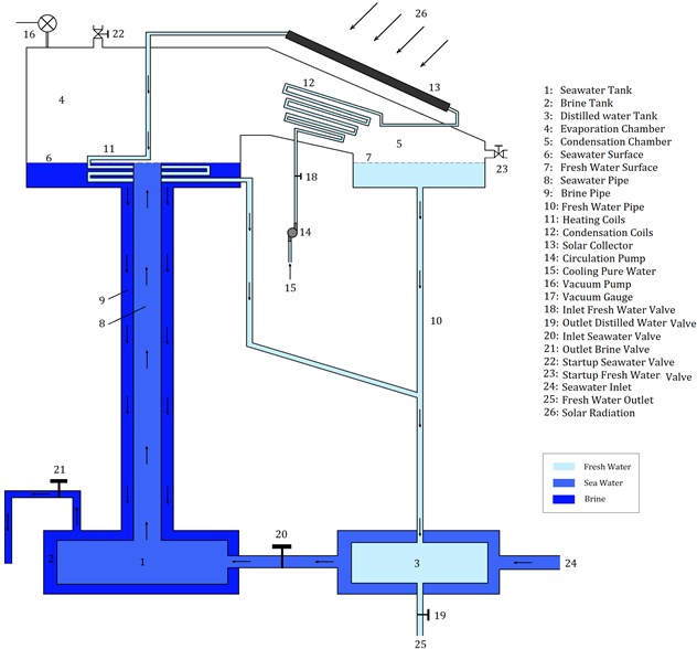
In this section, our own SNVD system is described. The schematic diagram of our proposed SNVD system is shown in Fig. 1. Seawater tank is connected to the evaporator inlet, and the brine tank is also connected to the evaporator outlet, by tow pipes (one pipe inside the other). These tow pipes perform as a tube-in-tube heat exchanger. Also, the seawater tank is place inside the brine tank, and this performs as heat exchanger (recovering the heat of brine exiting from the evaporator). This is a unique idea in our SNVD system. The outer tube (i.e., brine pipe) should be insulated, in order to prevent heat losses, and thus, seawater can recover the heat of brine as maximum as possible.
Before system startup, we should ensure that the system (evaporation chamber, condenser, and pipes) is air-tight, that means, no leakage and no air entering into the system. At system startup, the valve 21 is closed while valve 22 is open. The evaporator, seawater tank, brine tank and pipes 8 and 9 are filled with seawater using valve 22. Similarly, using valve 23, the condenser and fresh water side are filled with fresh water. This is the first step in startup phase. After doing this step, all valves must be closed, the vacuum pump is used to create a vacuum condition in the evaporator and condenser.
After startup the system will operate naturally. Flat Plate Collector (FPC) is used to supply heat required for heating seawater. The pipe of pure water after evaporator is inclined to prevent distilled water of obstructing pure water. The withdrawn water (brine) has a temperature which is higher than that of injected seawater, so the proposed system is designed to recover this heat from brine. Two flow-control valves (18 and 19) are used to regulate the water flow rates in the system. Another two valves (22 and 23) are used to startup the system and then, be closed during operation.
Fig. 1Schematic diagram of the proposed system
3. Mathematical modeling
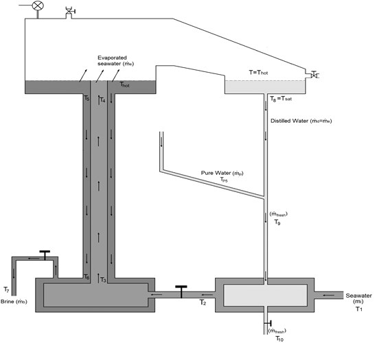
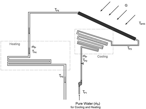
In order to do the modeling equations, we will consider two cycles. The first is seawater cycle (Fig. 2), which include the injected seawater, evaporated seawater, rejected brine, and distilled water. This cycle is discussed in details in Section 3.2. The second cycle is pure water cycle (see Fig. 4), which include the pure water used for cooling (in the condenser), and heating (in the evaporator). This cycle also includes the solar collector used to heat the pure water, and discussed in Section 3.3.
3.1. Vacuum parameters
As discussed earlier, after system startup, empty space is created in the top surface of seawater inside the evaporator. This empty space will be filled with vapor that evaporated from seawater, and then, pressure () corresponding to the seawater temperature is created. The value of is estimated from the follow equation [13]:
where is the saturated pressure corresponding to the seawater saturated temperature () at the top surface; is the atmospheric pressure; is the density of seawater; is the acceleration of gravity; and is the height of a seawater column that is required to create . The height () is given by:
We see that is a function of seawater temperature and salinity, since changes with seawater temperature, also changes with seawater temperature and salinity and was calculated from the correlations given by El-Dessouky and Ettouney [14] as:
where:
where, is the seawater density in kg/m3, is the salinity of seawater in ppm (parts per million), and is the temperature of seawater in ℃. The red sea is one of the most saline seas in the world. The salinity is about 41,000 ppm (41 g/kg). Also, the red sea is warm with temperature ranges from 20 ℃ to 31 ℃ [15]. In our calculations, we will consider the temperature of seawater entering the system to be 20℃. El-Dessouky and Ettouney [14] suggested an equation to calculate corresponding to :
where is in kPa and will be in ℃.
3.2. Evaporation calculations
The equation of mass conservation of seawater in the evaporation chamber is given by:
where is the mass flow rate of injected seawater (kg/s); is the rate of evaporated seawater (also called evaporation rate kg/s); is the mass flow rate of rejected seawater (also called brine kg/s). The parameters used in the equations of this section are shown in Fig. 2. The evaporating rate of seawater () is estimated from the excessive thermal energy () contained in seawater. In other words, when the temperature of heated seawater () become higher than the saturated temperature () by , the seawater contains an excessive thermal energy. This excessive thermal energy is given by [16]:
where is the specific heat of seawater (evaluated at ). Therefore, the amount of evaporated seawater, also called evaporation rate, is calculated as:
where is the specific enthalpy (kJ/kg) required to evaporate 1 kg of seawater at saturated conditions ( and ). The value of is determined using steam tables, or using the following equation suggested by [16, 17]:
Fig. 2Schematic diagram of the first cycle
The calculation of the specific heat of seawater depends on its temperature and salinity. In order to calculate it, we will use the following correlation suggested by El-Dessouky and Ettouney [14] as follow:
where:
where, is the salinity of seawater in (g/kg) or in (part per thousand). The amount of thermal energy () supplied by the FPC is calculated as:
where is the specific heat of pure water evaluated at . Due to this amount of heat, the seawater (inside the evaporation chamber) will acquire sensible and latent heats. The temperature of seawater will rise from to (sensible heat). Therefore, is given by:
where (= ) is the latent heat of evaporated seawater. Assuming that the evaporation chamber is well-insulated, the rate of heat losses is negligible. The surface area of the evaporator (for heat transfer) is given by:
where is the overall heat transfer coefficient in the evaporator; and is the Logarithmic Mean Temperature Difference and evaluated by considering the counter-flow. and are calculated as given in Eq. (13) and Eq. (14), respectively [17]:
The effectiveness of the evaporator tube is given in Eq. (15):
LMTD method is appropriate when the inlet and outlet temperatures are known. Therefore, this method is suitable to determine the size (surface area) of heat exchanger. When the outlet temperatures are unknown, it is difficult to use LMTD method. Therefore, -NTU method is preferred. The ε-NTU approach is used to study and analyze the performance of heat exchangers and also to predict the outlet temperatures of the working fluids [18]. -NTU approach is based on the effectiveness of heat exchanger. For our system, the effectiveness of the evaporator is given by:
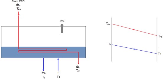
Fig. 3Energy balance on the evaporator
Another method used to estimate the temperature difference in heat exchangers is Arithmetic Mean Temperature Difference (AMTD). This method is preferred to avoid the complexity of LMTD method especially when the temperatures are unknown [18]. Eq. (12) can be written as:
where is calculated as [51]:
The brine has a salinity which is higher than that injected seawater. The salinity of brine () is calculated using Eq. (20). Since:
Therefore, salinity of brine is:
3.3. Condensation calculations
The pure water (), that is used to condense the evaporated seawater in the condenser, is preheated before entering the FPC. This pure water is preheated by absorbing the thermal energy of evaporated seawater (). This energy is the same value of excessive thermal energy estimated from Eq. (6). In other words, = , assuming that the evaporated steam is condensed completely. Therefore, the temperature of cooling pure water leaving the condenser (entering to the FPC) is calculated as:
where is the specific heat of pure water and we will evaluate it at . Because it is not important to use the exact value of , and to simplify the calculations, we will evaluate at .
The surface area of the condenser tube (for heat transfer) is given by:
where is the overall heat transfer coefficient in the condenser; and is the Logarithmic Mean Temperature Difference. and are calculated as given in Eq. (23) and Eq. (24), respectively [17]:
Fig. 4Schematic diagram of the second cycle
The effectiveness of the condenser tube is given in Eq. (25):
As mentioned in the previous section, we use -NTU method when the temperatures are unknown. For condensation calculations, Equ. (22) can be written as:
where is calculated as:
The effectiveness of the condenser is calculated using the ε-NTU method as following [18]:
where is the number of transfer units and we use Eq (29) to estimate :
3.4. Tanks and pipes calculations
The pure water leaving the evaporation chamber (with ) is mixed with the distilled water according to Eq. (30) and Eq. (31). After that, this fresh water is used to preheat the inlet seawater according to Eq. (32):
where is the rate of heat transfer in the fresh water tank. This amount of heat is transferred from the fresh water tank to preheat the seawater. Eq. (31) and Eq. (32) are then used to calculate the temperatures of fresh water () and seawater (), respectively. The tanks and pipes are treated as double-pipe heat exchangers with counter flow. The surface area of heat transfer in these is calculated as following:
where is the overall heat transfer coefficient in the fresh water tank which is calculated using Eq. (13) at ; and is the Logarithmic Mean Temperature Difference and is given by:
Arithmetic Mean Temperature Difference (AMTD) method may be used instead of LMTD. Then Eq. (33) can be written as:
where is calculated using Eq. (36) and the effectiveness of the fresh water tank is given in Eq. (37):
The inlet seawater inters the second tank with a temperature of and preheated again in this tank and the riser pipe. The amount of heat used for preheating the seawater in this stage ( plus ) is transferred from the brine that leaves the evaporator with a high temperature. The temperature of seawater increases from to in the seawater tank, then from to in the riser pipe. In the other hands, the temperature of the brine decreases to at the outlet of brine tank. The governing equations of this stage are the same manner of the fresh water tank. These equations are given below:
The values of and are determined using Eq. (13) at and , respectively. Arithmetic Mean Temperature Difference (AMTD) method may be used instead of LMTD. Therefore, Eq. (40) and Eq. (41) can be written as Eq. (44) and Eq. (45), respectively:
where and are given by Eq. (46) and Eq. (47), respectively. The effectivenesses of the seawater tank and pipes are given by Eq. (48) and Eq. (49), respectively:
3.5. Solar collector
In this study, FPC is used. The performance of solar collectors varies by the amount of solar radiation, the time and season and other factors such as wind velocity and the ambient temperature and. In order to evaluate the temperature of water exiting from the collector, we should use Eq. (52). The efficiency of FPC is the ratio of a thermal energy () gained by water (the working fluid) to the solar energy incident on the solar collector [19] and given by:
where is the mass flow rate of the pure water flowing in the collector; is the specific heat at constant pressure of the pure water flowing in the collector; is the outlet temperature of water from the collector; is the inlet temperature of water to the collector; is the effective area of an FPC; and is the solar irradiation per unit area. The efficiency of FPC varies by the temperature difference () between the working fluid and the ambient air (i.e., ). According to the review study by S. A. Kalogirou [20], the efficiency of FPC is inversely proportional to (i.e., increases linearly as decreases) as shown in Table 2. To find the efficiency of FPC at any value of and , we will use the following relation [19]:
Table 1Technical specifications of FPC
Collector type | Flat plate |
Model | SKR500 |
Gross area | 2.57 m2 |
Aperture area | 2.26 m2 |
Absorber area | 2.30 m2 |
Dimensions | 2079×1240×95 mm |
Collector capacity | 1.45 L |
Efficiency | 0.763 |
Heat transfer coefficient | 3.322 |
Temperature depending heat transfer coefficient | 0.018 |
For a given solar radiation, FPC area, water flow rate and inlet temperature, and ambient temperature, we can calculate the outlet temperature of water as:
Table 2Basic size and style requirements
, (°C) | ||
1000 W/m2 | 500 W/m2 | |
0 | 80 % | 80 % |
10 | 74 % | 65 % |
20 | 66 % | 52 % |
30 | 58 % | 38 % |
3.6. Evaporation ratio (ER)
The evaporation ratio (ER) is the ratio of the distilled water production. In other words, ER is the amount of distilled water to the amount of injected seawater. ER is given by:
3.7. Gain output ratio (GOR)
The gain output ratio (GOR) is the ratio between the latent heat of the evaporated seawater () and the supplied heat (). GOR is given by [21]:
3.8. Specific productivity (SP)
The specific productivity (SP) is the ratio of the distilled water in kg/h (kilograms per hour) to the heat supplied by the FPC in kW. SP is given by:
where is the rate of water produced (distilled water in kg/s) which is equal to the evaporation rate () as following:
3.9. Thermal efficiency
The thermal efficiency of the system, which is defined as the ratio of useful energy () to the solar energy input (), is calculated using Eq. (57). is the solar energy absorbed by the FPC, and given by Eq. (58):
3.10. Basic considerations for calculations
In order to initiate the calculations and get the results, we should consider some assumptions. These assumptions are summarized as follow:
1) Seawater properties: the temperature and salinity of seawater play important roles when designing the SNVD system. Seawater with high salinity has high density, and then lower height for the chambers is required. Also, the density and specific heat of seawater depends on the temperature and salinity. In our calculations, we considered the average properties of the Red Sea (i.e., 41,000 ppm and 20 °C).
2) Solar irradiation (): the operation of the proposed SNVD system depends on the solar energy and weather conditions. The solar radiation incident on the FPC and the ambient temperature vary along the day, therefore, the production of distilled water will be variable. In order to estimate the area of FPC required to heat the working fluid (pure water), we will consider average values for solar irradiation and ambient temperature (in 21th December) as 409 W/m2 and 27.5 °C, respectively (Uqu weather station).
3) All the evaporated seawater () is completely condensed and then converted into distilled water (). These considerations mentioned above are shown in Table 3.
Table 3Basic considerations used for calculations
No. | Description | Symbol | Value |
1 | The salinity of seawater | 41,000 ppm | |
2 | The inlet temperature of seawater | 20 °C | |
3 | Ambient temperature | 27.5 °C | |
4 | The temperature of pure water entering to the condenser | 20 °C |
3.11. Calculations methodology
The calculations required for designing the proposed SNVD system are done utilizing Engineering Equation Solver (EES) software. These calculations are done in two steps. The first step is the initial calculations, from which we want to determine the appropriate area of the FPC (), surface area of the evaporator and condenser ( and ), the height of evaporation and condensation chambers (), and the rate of pure water (). For this purpose, we, initially, assumed some conditions, for example, the seawater inside the evaporator is to be heated 15 °C above the saturation temperature (i.e., 15 °C). The other initial conditions assumed are listed in Table 4.
From the initial calculations, we can estimate the values of , , , , and . The second step is to use these values as additional inputs to determine all the parameters of our system. From these calculations we can analyze and study the performance of our system during the year. The performance of the system varies with time depending on the change in the solar irradiation () incident on the tilted solar collector. We should note that the basic considerations listed in Table 3 are used for both initial and analysis calculations.
Table 4Initial conditions assumed for initial calculations
No. | Description | Symbol | Value |
1 | The amount of water production | 10 liter/hour (0.00278 kg/s) | |
2 | Average solar irradiation | 409 W/m2 | |
3 | The temperature of seawater after fresh water tank | + 5 °C | |
4 | The temperature of seawater entering the riser pipe | + 20 °C | |
5 | The temperature of seawater entering the evaporation chamber | + 20 °C | |
6 | The temperature of seawater inside the evaporator | + 15 °C | |
7 | The temperature of pure water leaving the solar collector and entering the evaporator | + 10 °C | |
8 | The temperature of pure water exiting from the evaporator | + 5 °C | |
9 | The temperature of fresh water leaving the system |
4. Results and discussion
The numerical results are represented and discussed in this section. These results are obtained by executing the EES codes that include the mathematical equations given in Section 3. The results are reported in the form of figures and tables.
4.1. Summary of system sizing
The sizing of the proposed SNVD system is obtained by executing the initial calculations as discussed in Section 3.11 and based on the basic considerations and conditions in Table 3 and Table 4. The sizing of the system is summarized below, in Table 5, including the size of the evaporator, condenser, tanks, pipes, and solar collector, in addition, the amount of pure water () required for condensing and heating. The results of simulation are based on a constant injected seawater of 0.1 kg/s.
Table 5Summary of SNVD system sizing
No. | Description | Symbol | Value |
1 | The elevation of seawater surface inside the evaporator | 9.5 m | |
2 | The surface area of evaporator tube | 0.4 m2 | |
3 | The surface area of condenser tube | 0.2 m2 | |
4 | The surface area of fresh water tank | 0.5 m2 | |
5 | The surface area of seawater tank | 0.5 m2 | |
6 | The surface area of the riser pipe. | 0.5 m2 | |
7 | The effective area of the solar collector. | 23 m2 | |
8 | Mass flow rate of pure water | 0.12 kg/s |
4.2. Annual operation and performance simulation
The performance of the system is simulated hourly throughout the year. The distilled water production rate, , in kilogram per hour is shown in Fig. 5. The outlet temperature from the solar collector, , and the temperature of seawater inside the evaporator, , are shown in Fig. 6 and Fig. 7, respectively.
Fig. 5Distilled water throughout the year (kg/hour)
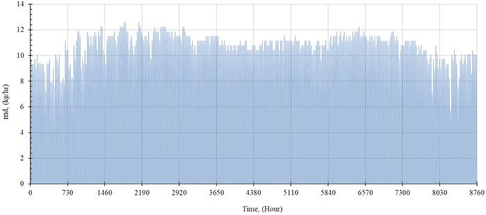
Fig. 6Outlet temperature from solar collector
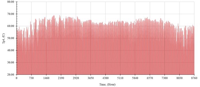
Fig. 7Temperature of seawater inside the evaporator
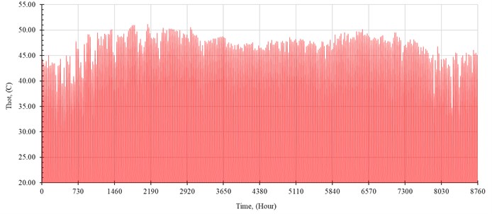
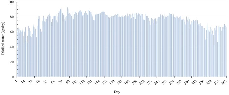
Fig. 8 represents the production rate of water per day throughout the year. The maximum production of distilled water is achieved during Spring season, especially in March and April. The production of our proposed system in that duration reaches 92.88 kg per day, which is equivalent to 2.13 % of the seawater injected. In addition, in summer season, the system achieves maximum gain output ratio (), specific productivity (), and thermal efficiency () of 0.98, 1.45 kg/kWh, and 39.6 %, respectively.
Fig. 8Daily distilled water and evaporation rate
The accumulated amount of distilled water per month exceeds 2500 kg in April, May and July. It reaches 2625 kg, as a maximum value of production, and is achieved in July, while in January the system produces minimum distilled water of 1861 kg. The production of water per month is shown in Table 6 and Fig. 9. Also, the monthly average evaporation ratio (), monthly average specific productivity (), and monthly average are represented in Table 6 and illustrated in Fig. 10 and Fig. 11.
Fig. 9Accumulated distilled water per month
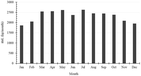
Fig. 10Monthly average evaporation ratio (ER) and monthly average specific productivity (SP)
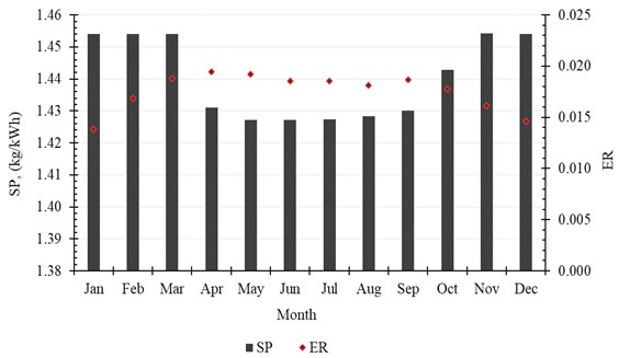
Fig. 11Monthly average GOR
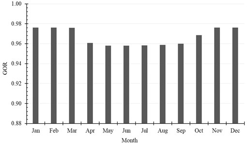
Table 6Monthly production of water
Month | , (kg/month) | ER | GOR | SP, (kg/kWh) |
January | 1860.84 | 0.0138 | 0.9762 | 1.4541 |
February | 2051.64 | 0.0169 | 0.9761 | 1.4540 |
March | 2541.24 | 0.0188 | 0.9760 | 1.4540 |
April | 2553.12 | 0.0195 | 0.9606 | 1.4310 |
May | 2612.16 | 0.0192 | 0.9580 | 1.4272 |
June | 2373.84 | 0.0185 | 0.9580 | 1.4271 |
July | 2625.48 | 0.0185 | 0.9582 | 1.4274 |
August | 2453.76 | 0.0181 | 0.9589 | 1.4284 |
September | 2443.32 | 0.0187 | 0.9600 | 1.4301 |
October | 2387.16 | 0.0177 | 0.9685 | 1.4427 |
November | 2087.28 | 0.0161 | 0.9762 | 1.4542 |
December | 1952.28 | 0.0146 | 0.9761 | 1.4541 |
4.3. Characteristics of the SNVD system
In order to analyze the performance of the SNVD system evidently, we executed a simulation for the system operation throughout a single day (21st December). All the parameters required for analyzing the performance are discussed in this section. These parameters comprise the temperatures, heat flow, efficiencies, evaporation rate and ER.
Fig. 12Temperatures in the first cycle
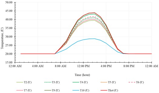
The temperature distribution along the first and second cycles are shown in Fig. 12 and Fig. 13, respectively. These figures show that the temperatures along the system increase with time as the irradiation increase until midday at which the solar radiation is peak value, then decreasing gradually with time. We can note, from these two figures, that all temperatures show the same trend, however, the outlet temperature from solar collector () shows a slightly different profile. This is because is affected strongly by solar radiation.
Fig. 13Temperatures in the second cycle
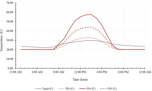
Fig. 14Heat flow and solar irradiation
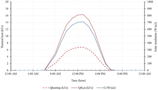
Fig. 15Accumulated distilled water in 21th December
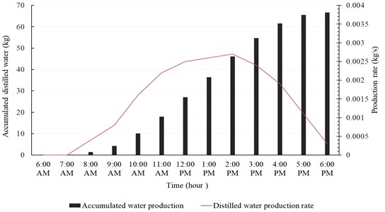
The useful heat () and the input heat () are represented in Fig. 14. The useful heat increases with time until peak value of 16.3 kJ/s at 1:00 PM, then decreases with time. Note that the useful heat () and the input heat () increase rapidly, with solar radiation, from 9:00 AM to 11:00 AM. The system produces maximum amount of distilled water at midday (12:00 AM-2:00 PM). The temperature of brine leaving the system () is relatively high compared to the temperature of injected seawater (). In addition, the temperature of pure water exiting the evaporation chamber () is relatively high compared to . Fig. 15 represents accumulated distilled water in 21st December and the instantaneous rate of water production.
5. Conclusions
SNVD system is one of the most promising solar desalination systems in which tow separated tanks are filled with seawater and fresh water. These tanks are vacuumed naturally by the gravity of water. The advantage of using this technique is the efficient use of low-grade heat sources such as solar radiation.
The proposed SNVD system is described and modeled theoretically utilizing the principles and equations of thermodynamics. Theoretical simulation is, then, executed hourly throughout the year based on the solar irradiation and some considerations. The outputs and results of simulation are illustrated in figures. From these results, it is obvious that the FPC with effective area of 23 m2 is sufficient to supply the heat required to provide, at least, 66.6 liter of distilled water per day in 21st December, which is the shortest day in the year. Maximum production of the proposed system would be in 30th March with 92.88 liter/day. Based on these values, the system would produce maximum amount of distilled water of 4.04 liter/m2/day. The proposed system is small-scale when compared with desalination plants, therefore, it is suitable to construct such system in remote areas where a large desalination plant installation is difficult or not feasible.
Further study and experimental modeling will be conducted to prove the theoretical results. In addition, further research and study will be conducted to improve the performance of the system as possible.
References
-
F. Tarrass and M. Benjelloun, “The effects of water shortages on health and human development,” Perspectives in Public Health, Vol. 132, No. 5, pp. 240–244, Sep. 2012, https://doi.org/10.1177/1757913910391040
-
S. Vaithilingam et al., “An extensive review on thermodynamic aspect based solar desalination techniques,” Journal of Thermal Analysis and Calorimetry, Vol. 145, No. 3, pp. 1103–1119, Aug. 2021, https://doi.org/10.1007/s10973-020-10269-x
-
H. Manchanda and M. Kumar, “Study of water desalination techniques and a review on active solar distillation methods,” Environmental Progress and Sustainable Energy, Vol. 37, No. 1, pp. 444–464, Jan. 2018, https://doi.org/10.1002/ep.12657
-
N. K. Nawayseh, M. M. Farid, A. A. Omar, and A. Sabirin, “Solar desalination based on humidification process-II. Computer simulation,” Energy Conversion and Management, Vol. 40, No. 13, pp. 1441–1461, Sep. 1999, https://doi.org/10.1016/s0196-8904(99)00017-5
-
F. Vince, F. Marechal, E. Aoustin, and P. Bréant, “Multi-objective optimization of RO desalination plants,” Desalination, Vol. 222, No. 1-3, pp. 96–118, Mar. 2008, https://doi.org/10.1016/j.desal.2007.02.064
-
A. Rashid, T. Ayhan, and A. Abbas, “Natural vacuum distillation for seawater desalination – A review,” Desalination and Water Treatment, Vol. 57, No. 56, pp. 26943–26953, Dec. 2016, https://doi.org/10.1080/19443994.2016.1172264
-
S. Al-Kharabsheh and D. Y. Goswami, “Experimental study of an innovative solar water desalination system utilizing a passive vacuum technique,” Solar Energy, Vol. 75, No. 5, pp. 395–401, Nov. 2003, https://doi.org/10.1016/j.solener.2003.08.031
-
G. A. Bemporad, “Basic hydrodynamic aspects of a solar energy based desalination process,” Solar Energy, Vol. 54, No. 2, pp. 125–134, Feb. 1995, https://doi.org/10.1016/0038-092x(94)00110-y
-
A. Midilli and T. Ayhan, “Natural vacuum distillation technique-Part I: Theory and Basics,” International Journal of Energy Research, Vol. 28, pp. 355–371, 2004.
-
A. Midilli and T. Ayhan, “Natural vacuum distillation technique-Part II: Experimental investigation,” International Journal of Energy Research, Vol. 28, pp. 373–389, 2004.
-
T. Jitsuno and K. Hamabe, “Vacuum distillation system aiming to use solar-heat for desalination,” Journal of Arid Land Studies, Vol. 22, pp. 153–155, 2012.
-
M. Reali, G. Modica, A. M. El-Nashar, and P. Marri, “Solar barometric distillation for seawater desalting part I: Basic layout and operational/technical features,” Desalination, Vol. 161, No. 3, pp. 235–250, Mar. 2004, https://doi.org/10.1016/s0011-9164(03)00704-5
-
Y. A. Cengel and J. H. Cimbara, Fluid Mechanics-Fundamentals and Applications. New York: McGraw-Hill, 2006.
-
Hisham T. El-Dessouky and Hisham M. Ettouney, Fundamentals of Salt Water Desalination. Amsterdam: Elsevier B.V., 2002.
-
https://www.Ioc.gov/everyday-mysteries/geography-anthropology-recreation/item/what-are-the-seven-seas/
-
S.-H. Choi, “On the brine re-utilization of a multi-stage flashing (MSF) desalination plant,” Desalination, Vol. 398, pp. 64–76, Nov. 2016, https://doi.org/10.1016/j.desal.2016.07.020
-
H. Ettouney et al., Fundamentals of Salt Water Desalination. Elsevier, 2002.
-
J. P. Holman, Heat transfer. 10th ed., New York: McGraw-hill, 2010.
-
“Sonnenkraft”. http://www.sonnenkraft.dk/
-
S. A. Kalogirou, “Solar thermal collectors and applications,” Progress in Energy and Combustion Science, Vol. 30, No. 3, pp. 231–295, 2004, https://doi.org/10.1016/j.pecs.2004.02.001
-
A. M. Abdel Dayem and A. Alzahrani, “Psychometric study and performance investigation of an efficient evaporative solar HDH water desalination system,” Sustainable Energy Technologies and Assessments, Vol. 52, p. 102030, Aug. 2022, https://doi.org/10.1016/j.seta.2022.102030
About this article

This study was supported by A.M. Abdel Dayem, Mechanical Engineering Department, College of Engineering and Islamic Architecture, Umm Al-Qura University, Makkah, P.O. 715, Saudi Arabia.
