Research of the dynamical properties of mechatronic prosthesis

1. Introduction

Prostheses for below-knee amputees are typically passively constructed mechanical structures with a major disadvantage to reproduce all the characteristics of the biological gait cycle – various studies have shown that the lack of ability to actively generate energy during a specific walking cycle period results in both general fatigue and possible health issues [1]-[3]. To address these problems, active prostheses for below-knee amputees were developed and are electrically controlled mechanical structures which are mostly orientated to reflect a typical walking gait where both kinematics and dynamics are taken as characteristics to be assumed [4]-[6]. The electrically active prostheses were initially developed to provide a positioning of the structure which was the most important aim for the active control – these types of structures showed a capability to set the structure position to the gait starting state [7], [8]. Since then, several various actively controlled prostheses were introduced mainly showing active-energy characteristics only for kinematics of the structure but not for the additive force generation that a biological limb is capable of [9], [10]. Types of control were related to resistance change, constrainment of elasticity, shift of the moment arm, etc. As technology developed the iBiom angle joint was introduced by H. Herr showing the efficiency of active system involvement in the overall gait and not only in the positioning as it was [5], [11], [12]. Controlled dynamics of the structure were seen both in kinematic characteristics (amplitudes of the movement, ability to change position in terms of gait patterns, etc.) and dynamics – the rate at which all preferable movement is reached [13]. Although the new development of active control implementation to the overall walking cycle was seen as a high improvement, the consequence of reducing the kinematic capabilities was introduced due to the complexity and the nature of the movement in the investigated joint [14], [15]. A need for complex design decisions reduced the level of a structure to meet its initial goal – to help regain the lost movement of the amputee. The kinematic capabilities of a prosthesis depend on various variables and design goals. The stability, strength and resistance of a structure, reliability, cost-effectiveness and design consistency are the factors that demand a simple structure while the increase in the level of natural movement reflection introduces the unpreferable complexity which is reflected in the degrees of freedom in the system [5], [13], [16].

Environmental conditions for a structure are also variables for the end-kinematics to be seen: level of activeness, a need for mobility, and the intensity of the disease can also affect the decision in design to be made.

All of these different variables act as additional complexity parameters thus introducing time-consuming, cost-inefficient and additional error factors [17]-[19]. Most of these are addressed in traditionally based calculation methods which not only shift the initial goal for a prosthetic to mimic the behaviour of a biological limb but also do not provide intuitively understood dynamics as are based on the static evaluation. Dynamic parameter evaluation demands a need for evaluation of a change rate in parameters to be seen. Time-domain change is a parameter from itself as a quotative value. The rate at which the parameter of the structure is changing can be misleading in terms of the value of the rate excluded from the overall picture. Actively controlled prostheses are highly change-rate dependent structures that do not base their initial behaviour only on static value characteristics [20], [21]. These time-dependent parameters are based on the environmental characteristics which are derived from the typical walking gait cycle [22], [23]. All time-dependent characteristics are the result which is seen as the rate of angular displacement over certain periods which are indicated by different phases of the structure's working cycle itself. These variable-based phases are differentiated into foot-on-ground and foot-off-ground types. The phase of interest in designing an actively controlled structure is the foot-on-ground phase with its own five sub-phases to be used as qualitative end-start areas with a particular displacement rate to be evaluated [9]. The structurally most intensive sub-phase of the foot-on-ground gait cycle phase is the additional force where the object of investigation should provide the highest amount of energy in the shortest period – the energy to time ratio is in its highest value [15], [24], [25]. Without a clear indication of whether the provided energy for this particular sub-phase is sufficient enough to reach a desired angular displacement after a certain time, major design flaws can be seen such as delayed energy provision, lack of work exceeded by the prosthetic and the overall disturbance of the gait cycle leading not on only to inefficient walking experience but also to probable additional health issued due to unsymmetric muscle work [26], [27]. All of these time-based energy solutions should be addressed in every degree of freedom to evaluate the effect of complex movement and the probability of additional energy losses both based on amplitude and change rate terms. A particular method for describing the needed rate-change parameters of the structure is related to the mathematical modelling techniques which describe the output of the actively affected system. The system chosen for a tool to be later used is validated with a physical model and later compared to the predictable dynamics of the structure with the derived tool.

The main aim of this work was to create a model for an actively controlled system evaluation in terms of dynamically changing characteristics of the structure under investigation. The resultant time domain parameters of the model should work as an indicative tool to design a structure including not only strength based but also rate change decisions. Model input parameters such as mass, torque, moment arm, etc. allow choosing qualitative design parameters for an individual structure as well as forecasting the probable dynamic behaviour of the structure of the investigation.

Results have shown a considerably high correlation ratio in terms of amplitude response for both force and displacement values, therefore a strong statement can be placed for further development research in the area of interest.

As there is no common practice to use mathematical models of such kind in the development of personalized prosthetics in the field of the gait rehabilitation process, the presented model has the potential to be used as a standardized tool for custom solutions of the actively controlled prosthetics.

This paper is composed of five general sections: Introduction, Modelling, Experiments, Results and discussion, and Conclusion. Modelling section covers methodology and simulation subsections. Experiments section is composed of theoretical background, methodology and error calculation subsections. Results and discussion section comprises modelling results, experimental results and comparison subsections.

2. Modelling

2.2. Model of mechanical system

The object of interest is comprised form the basic structural elements: a gear from two lead screws, two belt gears, two motors, an elastic element and other rotational joints. For simplicity of the mathematical model derivation, a symmetrical modelling approach is used to derive a system representing half of all the components as all stiffness, damping and mass parameters are used to cover the overall structural elements and the behaviour of interest.

Fig. 1The modelled object of interest – a mechatronic ankle prosthesis

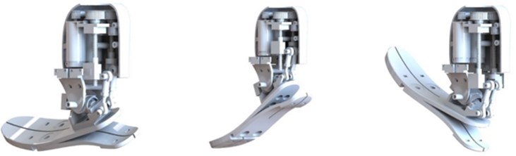
All-important structural parts of the modelled mechatronic prosthesis are replicated with dedicated mass for each part while the stiffness and damping effects are represented with individual springs and dampers for stiffness and dampening. All the dedicated parameters for each element are given in Table 1. The general idea behind the mass-spring model covers the activation of the motor by transferring rotational movement through the belt gears to the pulleys which are rigidly connected to the lead screw. The later movement of the lead nut is described as the movement with dampening due to the inertia of the motor’s rotor. The movement from the lead nut is then transferred to the deformation of the flexible foot as the additional constrainment comes from the parallel spring. The affected foot element through the rotational joint of the ankle is transferring movement to the ground.

Equations of motion were derived for both vertical and horizontal movement as given below. The general equations for vertical movement are:

2

$m_4{\ddot{x}}_4+k_3{x}_4+b_1{\dot{x}}_4-k_3{x}_5=F,$

3

$m_5{\ddot{x}}_5+k_3{x}_5+k_4{x}_5+k_5{x}_5+k_6{x}_5-k_3{x}_4=0.$

The general equations for horizontal movement are:

4

$\left(m_2+m_3\right){\ddot{x}}_{\frac{2}{3}}+k_1{x}_{\frac{2}{3}}+k_2{x}_{\frac{2}{3}}-k_2{x}_4=F,$

5

$m_4{\ddot{x}}_4+k_2{x}_4-k_2{x}_{\frac{2}{3}}=0.$

Fig. 2Mass-spring-damper system of the modelled mechatronic ankle prosthesis

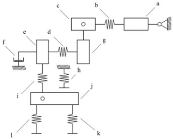
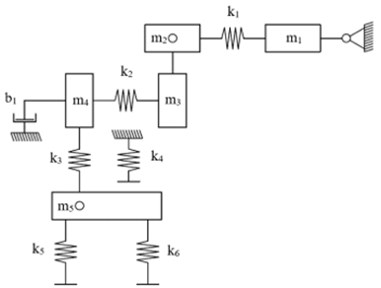
Table 1Parameters and indication of components used for mass-spring-damper system

Component	Description	Indication	Value	Units
a	Motor	$m_1$	0.325	kg
b	Motor-belt joint stiffness	$k_1$	244	N/m
c	Belt-gear pulley	$m_2$	0.034	kg
d	Lead screw-nut stiffness	$k_2$	1500	N/m
e	Lead-screw nut	$m_4$	0.12	kg
f	The inertia of the rotor	$b_1$	0.31	Ns/m
g	Lead-screw	$m_3$	0.094	kg
h	Spring stiffness	$k_4$	330	N/m
i	Stiffness of the end-foot	$k_3$	1200	N/m
j	Stiffness of the front-foot	$m_5$	0.542	kg
k	Stiffness of the bottom foot	$k_6$	1200	N/m
l	Stiffness of the heel	$k_5$	1200	N/m

3. Simulation

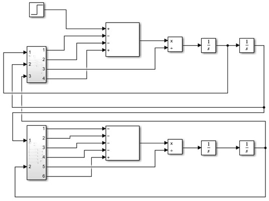
Simulation of the representative mass-spring-damper systems is implemented with the Matlab Simulink software in which all the parts of the modelled object of interest are represented by the dedicated mathematical block which in turn represents the equation of motion.

The derived equations for the computational model for the vertical movement are:

The derived equations for the computational model for the horizontal movement are:

Fig. 3Matlab Simulink model for movement in the vertical and horizontal directions

4. Experiments

4.2. Methodology

For the test of the generated force of the object of interest a force plate, BTS P-6000 is used. The dedicated reaction force measurements were taken for the plantarflexion motion as the measured force is later compared with the calculated acceleration of the foot mass from the mathematical model. For the ankle joint angular movement (both displacement and velocity) two approaches are implemented – angular displacement measurement with MP6050 gyroscopes and using potentiometers placed on every rotational joint of the structure of the investigation. All measurements were taken with three configurations: at the neutral position (N) (ankle rotation in the frontal plane is 0 deg), at the highest inversion position (IN) (ankle rotation in the frontal plane is –15 deg) and at the highest eversion position (EV) (ankle rotation in the frontal plane is 15 deg). There were 10 samples taken for each plantarflexion movement in each configuration as mentioned before. All general technical specifications are given in Table 2.

Table 2Technical specification of the used instruments

	BTS P-600	MP6U050	Potentiometer
Sampling frequency	500 Hz / 1000 Hz	500 Hz	10 kHz
Range	–8000 N – 8000 N	360 deg	300 deg
Resolution	0.12 N (16 bit)	0.35 deg (10 bit)	0.29 deg (10 bit)
Deviation	2 %	1.75 deg	1.45 deg

Fig. 4The object of interest on the BTS P-6000 force plate

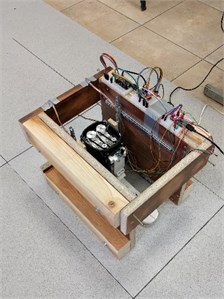
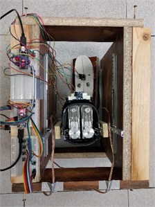
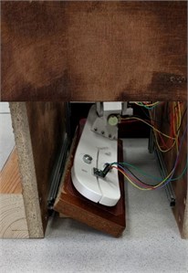
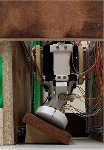
Fig. 5The object of interest with MPU6050 and potentiometers sensors

5. Results and discussion

5.3. Comparison

Comparison is given in form of plots for both experimental results and outputs of the mathematical model. For every given plot a dedicated table indicates the error and difference for amplitude value, response time and time to reach the amplitude value. For every test, standard deviation and variance values are also shown to inspect the validity of experimental results.

5.3.1. Force comparison

Fig. 6Comparison plots between simulated and test results, acceleration

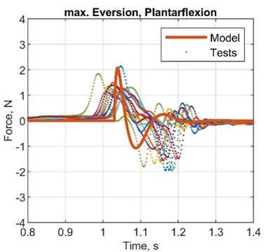
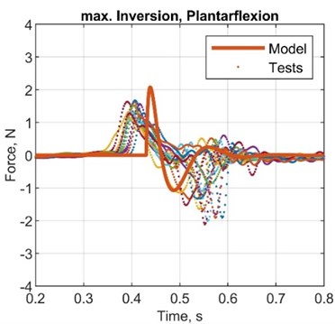
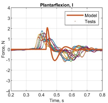
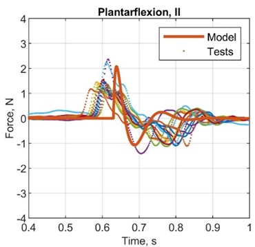
Table 7Comparison between simulated and test results, acceleration

	1st plot	2nd plot	3rd plot	4th plot
AMP diff., N	0.30	0.50	0.50	0.80
ST diff., s	–0.20	–0.25	-0.30	–0.32
AMP. T diff., s	–0.15	–0.05	0.03	–0.01
AMP error, %	16.7	31.3	31.3	61.5
ST error, %	–50.1	–55.6	–60.1	–61.1
AMP. T error, %	–75.1	–50.4	150.2	–16.5
STD, N	0.27	0.32	0.32	0.35
VAR, N2	0.62	0.84	0.89	1.03

5.3.2. Angular displacement comparison (MPU6050)

Fig. 7Comparison plots between simulated and test results, angular displacement (MPU6050)

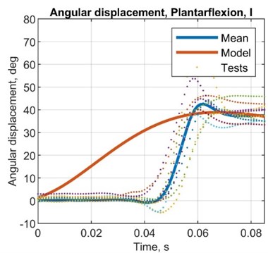
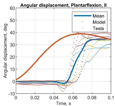
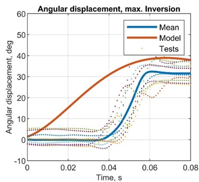
Table 8Comparison between simulated and test results, angular displacement

	1st plot	2nd plot	3rd plot	4th plot
AMP diff., deg	–4.00	3.00	7.00	6.00
AMP R. diff, deg	–6.00	–2.00	3.00	1.00
ST diff, s	0.14	0.17	0.16	0.16
AMP T. diff, s	0.03	0.02	0.03	0.03
AMP error, %	–9.52	8.57	22.6	18.8
AMP R. error, %	–15.8	–5.88	10.3	3.23
ST error, %	233.3	566.7	395.5	499.1
AMP T. error, %	150.2	66.7	149.1	148.3
STD, deg	2.61	3.48	2.62	3.19
VAR, deg2	0.07	0.12	0.07	0.10

5.3.3. Angular displacement comparison (potentiometer)

Fig. 8Comparison plots between simulated and test results, angular displacement (potentiometer)

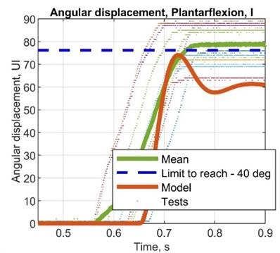
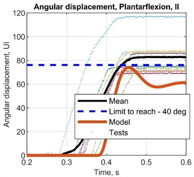
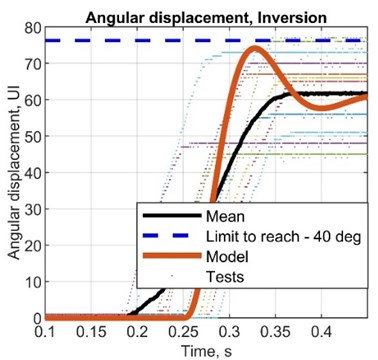
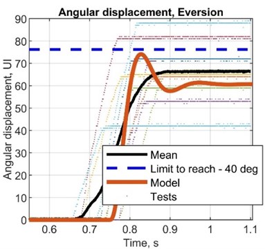
Table 9Simulated values for displacement and calculated for angular displacement

	1st plot	2nd plot	3rd plot	4th plot
AMP diff., deg	–3.00	–13.1	10.4	14.1
AMP R. diff, deg	–16.1	–26.5	–3.32	1.12
ST diff, s	–0.05	–0.05	–0.10	–0.02
AMP T. diff, s	–0.20	–0.20	–0.25	–0.17
AMP error, %	–3.85	–14.8	15.3	22.9
AMP R. error, %	–20.5	–29.6	–4.62	1.64
ST error, %	–20.4	–20.8	–33.3	–9.09
AMP T. error, %	–80.2	–80.6	–83.5	–77.2
STD, deg	6.86	7.65	5.52	5.89
VAR, deg2	2.38	3.00	1.57	1.80

5.3.4. Angular velocity comparison

Fig. 9Comparison plots between simulated and test results, angular velocity

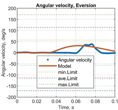
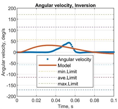
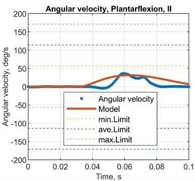
Table 10Comparison between simulated and test results, angular velocity

	1st plot	2nd plot	3rd plot	4th plot
AMP diff., deg/s	–30.2	–6.12	–8.15	–16.1
ST diff., s	0.14	0.15	0.16	0.15
AMP. T diff., s	0.02	0.02	0.04	0.03
AMP error, %	–48.4	–15.8	–20.1	–33.3
ST error, %	233.3	295.1	388.1	295.4
AMP. T error, %	42.9	66.7	233.3	149.2

6. Conclusions

Here established mathematical model is suitable to determine the characteristics of the dynamic behaviour of the object of interest – the mechatronic system of the actively controlled prosthesis. Simulated results showed the same pattern behaviour in terms of both amplitude and response time. Experiments were conducted for three different configurations for the most demanding sub-phase of the system (plantarflexion) covering nominal, highest amplitude inversion and eversion positions. Three parameters – angular displacement, angular velocity and angular acceleration – were compared by calculating differences and errors for amplitude, response time and time to reach the favourable value of the parameter under interest. Comparison of acceleration of the joint was conducted through exerted force values as the error at the plantarflexion reached 24.1 %, –52.9 % and –62.8 % for the amplitude, response time and time to reach the highest amplitude, respectively. Corresponding errors at the inversion and eversion positions showed values of 46.4 %, 60.6 % and –16.7 %. Angular displacement error values for amplitude, reached displacement, response time and time to reach the amplitude have shown –9.1 %, –10.8 %, 482.1 % and 180.5 %, respectively. Corresponding error values for positions in inversion and eversion reached 20.7 %, 6.8 %, 447.3 % and 148.7 %. Values from the potentiometer showed errors of –9.3 %, –25.1 %, –20.6 % and –80.4 %. Angular speed comparison has indicated the error of –32.1 %, 264.2 % and 54.8 % as for positions in inversion and eversion –26.7 %, 341.8 % and 191.3 % were reached. In respect of the calculated error values, the amplitude response seems to have the closest representative behaviour as the response time in terms of angular displacement and velocity does not indicate a high correlation ratio. The overall patterns of the exerted force seem to replicate the calculated one by the mathematical model as the simulated response of the angular displacement and angular velocity are a good indicator only in terms of the amplitude value.