Fault diagnosis method of high voltage circuit breaker based on the combination of time-frequency multi-characteristics of acoustic signal

1. Introduction

Circuit breaker is one of the most important equipment to ensure the stable operation of power system. According to the statistics at home and abroad, mechanical fault is the main fault of circuit breaker, accounting for more than 80 % [1]. Vibration signal is often used as an important carrier of its state information [2, 3]. However, limited to the charge accumulation effect and coupling mode of piezoelectric acceleration sensor, it is easy to cut the top when the amplitude is large, and it has high requirements for the installation position of the sensor [4]. In addition, “the code for the management of high voltage switchgear (SGS[2004]No. 634)” stipulates that it is prohibited to place other devices that may affect the operation on the operating equipment. Therefore, it is of great significance to explore a non-contact in vitro monitoring method.

The acoustic signal that accompanying the circuit breaker operation is homologous with the vibration signal, which can be obtained by the non-contact electret thin film capacitive sensor. The measurement frequency band is wide, which can effectively avoid the phenomenon of roof cutting [5]. Moreover, the sensor is easy to install, the signal is less affected by the installation mode, and the field practicability advantage is obvious.

For non-stationary signals such as acoustic signal, dynamic time warping (DTW), wavelet transform (WT), empirical mode decomposition (EMD) and local mean decomposition (LMD) are often used for processing [6-9]. DTW is prone to abnormal distortion in optimal path planning, and WT has the problem of energy leakage. EMD and LMD belong to recursive decomposition method in principle, and modal aliasing and false modes are very easy to occur in the iterative process [10]. Variational mode decomposition (VMD) is a non-recursive adaptive signal decomposition method proposed by K. Dragomiretskiy et al. [11]. After signal decomposition, multiple natural modes around the central frequency can be obtained, which has good noise robustness. It can effectively avoid the defects of EMD and other algorithms (such as mode aliasing) and improve the accuracy of signal decomposition [12]. However, the above decomposition methods are all aimed at vibration signals, and the research and processing of acoustic signals is still in a blank stage to a certain extent.

Using the acoustic signal to discriminate the state of the circuit breaker, some scholars have carried out related research. Reference [13] uses the K-S method try to search for the amplitude difference interval between the normal signal and the abnormal signal, and extracts the difference amplitude as a feature vector, and realizes the diagnosis of mechanical faults of circuit breakers by analyzing some features with the greatest contribution. Reference [14] extracts the cepstral coefficients of the gamma pass filter, the Mel cepstral coefficients, and the power-law normalized cepstral coefficients of the acoustic signal to form the mixed cepstral coefficients, which are input to the convolutional neural network for fault identification. The above studies are all aimed at single-space processing, overemphasizing the time-domain or frequency-domain characteristics of the signal, splitting the connection between the eigenvectors and the original signal, making it difficult to form an effective and stable criterion, making the state identification less reliable. Therefore, how to effectively extract the time-frequency features becomes the key to the state identification of high-voltage circuit breakers.

In this paper, a new diagnostic method of acoustic signal time-frequency joint is proposed. After preprocessing the acoustic signal, the time-domain waveform index and frequency-domain spectral entropy are extracted to construct joint multi-characteristics. Kenerl fuzzy $c$ means – support vector machine (KFCM-SVM) classification and recognition algorithm are used to comprehensively analyze the state of high-voltage circuit breaker, and the effectiveness of the proposed method is verified by experiments.

2. Fault diagnosis process

The working environment of the circuit breaker is complex, and the acoustic signal is mixed with environmental noise and other equipment operation noise. Therefore, this paper establishes a background noise library for template matching to remove the template noise, and then uses adaptive wavelet transform (AWT) to remove the residual noise.

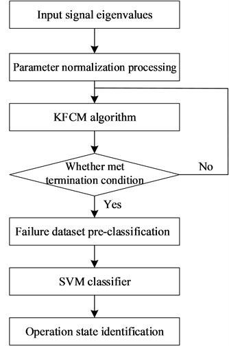
The operation process of the circuit breaker is controlled by electricity, from mechanical transmission to the release of elastic potential energy. The action of each component generates impact energy, so the acoustic signal reflects non-stationarity. The spectral characteristics of the signal frequency-domain are directly related to the operating state of the circuit breaker. Therefore, the denoised signal is gradually disassembled through VMD to obtain the spectrum, and the sensitivity to the main peak in the frequency domain is enhanced by the divergence factor, and the spectral difference entropy characteristic is obtained. At the same time, in order to improve the reliability, the time-domain waveform index of the original signal is introduced to construct the time-frequency joint features. The KFCM model is used to establish the membership mapping between the original sample feature sets and the fault types, so as to realize the pre-classification of the original data sample features of the circuit breaker. Based on the clustering results, the SVM classifier is trained for classification, and the final identification result is obtained after comprehensive evaluation. The diagnostic process is shown in Fig. 1.

Fig. 1Circuit breaker fault diagnosis process

3. Background noise library combined with AWT denoising

The working environment of the circuit breaker is poor. The operation site is mixed with environmental noise such as wind, thunder, steam whistle and human voice, as well as operation noise such as switching of air-cooling device and corona discharge. The template noise library is established by collecting background noise samples. Firstly, the zero-crossing energy product of the acoustic signal is obtained to detect the starting point, and then the spectral centroid is obtained by using the short-time Fourier transform (STFT), and finally the Gaussian mixture model (GMM) is used for template sample similarity matching removes background noise.

The spectral centroid reflects the fundamental attribute of the timbre, which is the weighted average of the component amplitudes after STFT processing. The process is as follows:

where $A_i\left[n\right]$ is the amplitude value.

GMM uses the combination of Gaussian probability density function to represent multi-dimensional features. Firstly, it needs to cluster the spectral centroid, then calculate the Gaussian distribution parameters and weights as the initial value, and then establish GMM through iterative calculation. Finally, compare the calculation probability of the features to be divided with GMM one by one, and the highest output is the target feature, so as to remove the noise. Specific methods can refer to literature [15].

Due to the limited template and residual noise, an adaptive wavelet transform (AWT) denoising method is introduced in order to preserve the singular characteristics of the signal to the greatest extent. A new threshold function is proposed in AWT, which can realize the smooth transition of the shrinkage coefficient of the critical area, meet the denoising index and retain the key features at the same time. The expression of adaptive threshold is as follows:

where $x$ is the acoustic signal, $yz$ is the threshold and $M$ is the parameter. When $M$ is 1, Eq. (2) is transformed into soft threshold, and when $M>$ 10, Eq. (2) is close to hard threshold.

In order to increase the wavelet coefficients in the critical area, $M$ is selected by the energy distribution method to achieve adaptive filtering. The mathematical model is as follows:

where $E_{d_j}={\sum }_{k=0}^{N-1}{d}_{j,k}^2$. According to the wavelet decomposition theory, the decomposition energy of $d_1$ scale signal is closest to the noise energy, so $E_{nj}=2{\sum }_{k=0}^{N-1}{d}_{1,k}^2$ can be obtained. When the value of $M$ changes, the soft and hard smooth adjustment of the threshold function can be realized.

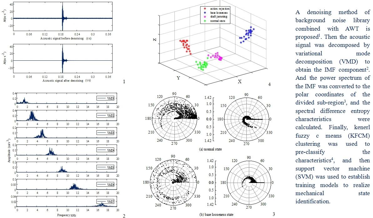
In this paper, the acoustic signal of ZN65-12 circuit breaker is denoised, and the results are shown in Fig. 2.

Verified by Fig. 2 and multiple groups of actual signals, the background noise of the acoustic signal after denoising is significantly reduced, and the local peaks of the signal are effectively preserved. The calculated signal-to-noise ratio is 35.03 dB, and the mean square error is 0.012. The denoising index is better than the soft and hard threshold denoising, which provides a strong guarantee for the accurate state identification of the circuit breaker.

Fig. 2Comparison of results before and after denoising in normal state

4. Time-frequency characteristics extraction

Time-domain and frequency-domain are the basic characteristics of acoustic signal changes. The abnormal state of circuit breaker can be found through scientific features comparison.

4.2. Entropy characteristics of frequency-domain spectrum

4.2.1. VMD algorithm

VMD is mainly divided into two parts: the establishment and solution of variational constraint problem. For the acoustic signal with data length $N$ in the operation process, the following problems are solved:

7

$\left\{\begin{array}{l}\underset{\left\{u_k\right\},\left\{{\omega }_k\right\}}{\mathrm{m}\mathrm{i}\mathrm{n}}\left\{{\sum _k‖{\partial }_t\left[\left(\delta \left(t\right)+\frac{j}{\pi t}\right)*{\mu }_k\left(t\right)\right]e^{-j{\omega }_{k}t}‖}^2\right\},\\ s.t.\sum _k{\mu }_k=f,\end{array}\right.$

where $\left\{{\mu }_p\right\}=\left\{{\mu }_1,\dots ,{\mu }_p\right\}$ is the decomposed $P$ modes, and $\left\{{\omega }_p\right\}=\left\{{\omega }_1,\dots {\omega }_p\right\}$ is the center frequency of the $P$ modes.

Lagrange multiplier $\lambda \left(t\right)$ is introduced to transform the above constrained variational problem into unconstrained variational problem:

8

$L\left(\left\{{\mu }_k\right\},\left\{{\omega }_k\right\},\lambda \right)=\alpha {\sum _k‖{\partial }_t\left[\left(\delta \left(t\right)+\frac{j}{\pi t}\right)*{\mu }_k\left(t\right)\right]e^{-j{\omega }_{k}t}‖}_2^2+{‖f\left(t\right)-\sum _k{\mu }_k\left(t\right)‖}_2^2$
$+⟨\lambda \left(t\right),f\left(t\right)-\sum _k{\mu }_k\left(t\right)⟩,$

where: $\alpha$ is the bandwidth parameter.

The saddle point of Eq. (8) is solved by ADMM method to continuously update ${\mu }_k^{n+1}$, ${\omega }_k^{n+1}$, ${\lambda }^{n+1}$, in which the modal component ${\mu }_k$ and center frequency ${\omega }_k$ are obtained as follows:

9

${\widehat{\mu }}_k^{n+1}\left(\omega \right)=\frac{\widehat{f}\left(\omega \right)-\sum _{i\ne k}{\widehat{\mu }}_k^n\left(\omega \right)+\frac{\widehat{\lambda }\left(\omega \right)}{2}}{1+2\alpha {\left(\omega -{\omega }_k\right)}^2},$

10

${\omega }_k^{n+1}=\frac{{\int }_0^{\infty }\omega \left|{\widehat{\mu }}_k^n\left(\omega \right)\right|\mathrm{d}\omega }{{\int }_0^{\infty }\left|{\widehat{\mu }}_k^n\left(\omega \right)\right|\mathrm{d}\omega }.$

VMD method steps are as follows:

1) Initialize ${\widehat{\mu }}_k^1$, ${\omega }_k^1$, ${\widehat{\lambda }}^1$, $n$, so that its initial value is 0, set the decomposition mode number $K$ to 2, and pre-decompose for optimization.

2) Update ${\mu }_k$ and $w_k$ respectively according to Eq. (9) and Eq. (10).

3) Update $\widehat{\lambda }$:

11

${\widehat{\lambda }}^n\left(\omega \right)+\tau \left[\widehat{f}\left(\omega \right)-\sum {\widehat{u}}_k^{n+1}\right]\to {\widehat{\lambda }}^{n+1}\left(\omega \right).$

4) If the following formula is satisfied, stop the iteration and output the result; Otherwise, return to step 2):

12

$\frac{{\sum ‖{\widehat{\mu }}_k^{n+1}-{\widehat{\mu }}_k^n‖}_2^2}{{‖{\widehat{\mu }}_k^n‖}_2^2}<\epsilon ,$

where: $\epsilon$ represents convergence accuracy.

4.2.2. VMD parameter $\mathbf{K}$ optimization

In order to prevent over decomposition of VMD, the $K$ parameter is selected according to the energy conservation theory before and after decomposition. For the denoised acoustic signal sequence $x\left(i\right)$ in Section 2, the energy calculation formula is as follows:

13

$E=\sqrt{\frac{\sum _{i=1}^n{x}^2\left(i\right)}{n}},$

where: $E$ is the signal energy value, and $n$ is the sampling point. In order to characterize the energy difference before and after VMD decomposition, the energy difference parameter $\psi$ is defined and calculated as follows:

14

$\psi =\frac{\left|\sum _{\mathrm{x}=1}^K{E}_x-E\right|}{E}\times 100\mathrm{\%},$

where: $E_x$ corresponds to the energy of the $x$-th component, $K$ is the number of components, and $E$ is the energy of the original signal. The energy is constant before and after decomposition (the ideal value is 0). After many experiments and calculations, the change trend of $K$ is shown in Fig. 3.

Fig. 3Change trend of parameter K

It can be seen from Fig. 3 that when $K$ is greater than 7, the energy difference parameter $\lambda$ increases, which can judge that there is over decomposition. At this time, the value $K$ at the turning point is the optimal decomposition mode number of VMD. The time-frequency diagram obtained by decomposing the acoustic signal in shaft jamming is as follows.

Fig. 4VMD time-frequency diagram of acoustic signal

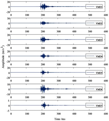
a) VMD diagram in time-domain

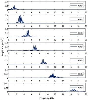
b) VMD diagram in frequency-domain

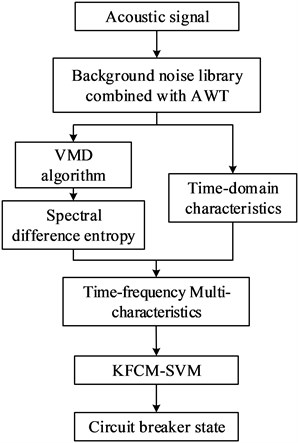
In order to verify the effectiveness of the VMD method, the author performs HHT (the core of which is EMD) processing on the acoustic signal, the frequency spectrum of IMF component after decomposition is shown in Fig. 5, in which 6 IMF components and 1 residual component are obtained through EMD adaptive decomposition.

Comparing the frequency spectra of VMD and EMD, it can be seen that the IMF frequencies after VMD decomposition are concentrated near their central frequencies, which effectively suppresses the problem of modal aliasing and false components after EMD decomposition. While reducing signal energy leakage, accurate characteristics are provided.

Fig. 5EMD time-frequency diagram of acoustic signal

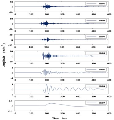
a) EMD diagram in time-domain

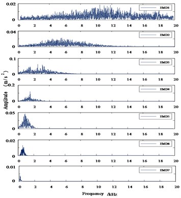
b) EMD diagram in frequency-domain

4.2.3. spectral difference entropy

After VMD decomposition, the frequency-domain spectrum of acoustic signal still has strong aggregation, which can not accurately describe the equipment state information contained in it. Therefore, a spectral difference entropy is proposed in this paper. The waveform is diverged by the divergence factor $\gamma$ to improve the sensitivity to the main peak area. According to the concept of the information entropy theory that events with a smaller probability of occurrence contain a larger amount of information, the spectral difference entropy is used to quantify the signal power distribution and spectral morphological characteristics. The calculation steps are as follows:

1) In polar coordinates, according to the polar diameter scale $\omega$ and the polar angle scale $d$, the polar coordinates are radially divided into several equal area sub-regions with the pole as the center, and the division formula is:

15

$a_{\omega }=a\times \left(\sqrt{\omega }-\sqrt{\omega -1}\right),$

16

$N=\omega \times d.$

Among them, $d$ and $\omega$ are integers, $d$ is the number of segments that the polar angle be divided equally, $a$ is the base value for dividing sub-regions in the polar radial direction, $\omega$ represents the number of segments divided in the polar radial direction; $a_{\omega }$ is the length of each segment in the polar radial direction; $N$ is the total number of divided regions in polar coordinates.

2) The frequency and amplitude $\left(f_i,h_i\right)$ of the power spectrum waveform in Cartesian coordinates are diverged in polar coordinates $\left(t_i,{\theta }_i\right)$ by the divergence factor $\gamma$:

17

$t_i=\sqrt{h_i^2+f_i^2},$

18

${\theta }_i=\gamma \times \mathrm{t}\mathrm{a}{\mathrm{n}}^{-1}\left(\frac{h_i}{f_i}\right).$

When $\gamma$ is 4, the power spectrum waveform that originally existed only in the range of 0-90° pole angle is extended to 0-360°, and the pole radial diameter remains unchanged.

3) The probability function of information entropy is constructed based on the frequency of waveform dispersion in the sub-region, which is redefined as the spectral difference entropy characteristics of perceived waveform variation and power main peak distribution in polar coordinates. The calculation formula is as follows:

19

$F=\sum _{i=1}^N\frac{p_i}{N}\times \mathrm{l}\mathrm{o}{\mathrm{g}}_2\frac{p_i}{N},$

where $p_i$ is the frequency of the waveform scattered in the $i$-th sub-region.

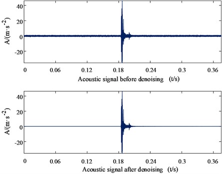
In this paper, the coordinates of seven modal components (IMF) decomposed by VMD are normalized by range method, and the maximum value is $\sqrt{3}$. If $a=$ 0.316 and $d=$ 24, then $\omega =$ 30, the polar coordinates are divided into 720 equal area sub regions. Using the sample library data in Section 5.1, select the first two orders of IMF power spectrum waveforms in normal state and base looseness state, as shown in Fig. 6 (IMF1 on the left and IMF2 on the right).

Fig. 6Polar coordinates of the power spectrum of the first two IMF components

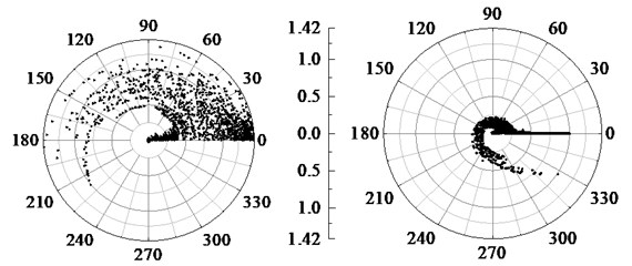
a) Normal state

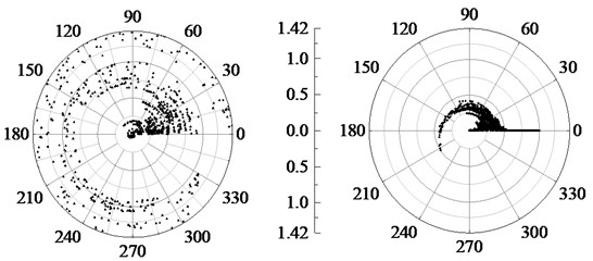
b) Base looseness state

The points with smaller amplitude in the power spectrum are limited near the zero pole axis, and the points with larger amplitude rotate and diverge counterclockwise along the zero axis, which reduces the probability of the data in the main peak region scattered in the same sub-region, so as to enhance the sensitivity and make the differential entropy characteristics of the circuit breaker spectrum have a specific distribution among various states.

5. KFCM-SVM identification model

Kernel based fuzzy c-means (KFCM) clustering algorithm introduces kernel parameters on the basis of fuzzy c-means (FCM) clustering, maps the samples in high-dimensional space, amplifies the feature differences between samples, and improves the clustering effect [16].

The objective function of KFCM uses the kernel function to replace the distance function in FCM, which is defined as follows:

where: $c$ is the number of classifications, $v_i$ is the cluster center of class $i$, $u_{ik}$ is the membership of the $k$-th sample to class $i$, and $K\left(v_i,x_k\right)$ is the Gaussian radial basis function:

According to the Lagrange multiplier optimization method to solve the minimum value of the objective function, the iterative formulas of $U$ and $V$ are derived as follows:

When there is $i\left(1\le i\le c\right)$ and $\sum _{j=1}^n{u}_{ij}=0$ holds, the iteration is stopped.

In this paper, the feature sets are pre-classified by KFCM, and the membership map between the feature sets and the fault categories is established. On this basis, the SVM is used for training, and the final result is obtained by comprehensive evaluation. The algorithm flow is as follows.

Fig. 7KFCM-SVM diagnosis process

6. Experimental results and analysis validation

6.1. Establishment of sample database

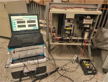
Since vacuum circuit breakers are mostly used in production sites (especially 10 kV systems), this paper takes ZN65-12 circuit breakers as an example to establish a high-voltage circuit breaker operation and fault simulation experimental platform. The platform is mainly composed of a sound sensor, a Hall current sensor, a signal acquisition device, a host computer and so on. The device diagram is shown in Fig. 8.

The sound sensor adopts F51 high fidelity pickup (frequency range 20 Hz-20 KHz) of huivocal music company, which is placed 30cm away from the circuit breaker. The clamp current sensor clamps the control coil and triggers signal acquisition. The upper computer is equipped with AMD I5-8250U processor, the main frequency is 3.4GHz, 14 “HD TFT LCD1920×1680 resolution, 64G solid state disk, 8GB/DDR4L memory, Intel® UHD Graphics 620GPU.

In addition to the normal signal samples, this paper also simulates several common faults of the circuit breaker: adjust the iron core gap so that the limit cushion cannot be fired, simulate the action rejection state; the wooden board is stuck on the rotating shaft to increase damping, simulate the shaft jamming state; pad a corner of the circuit breaker to simulate the base looseness state. The sampling frequency is set to 40 kHz, and 20 opening and closing experiments are carried out respectively.

Fig. 8Experiment and fault simulation platform

6.2. Experimental results

The time-frequency joint eigenvector is constructed by using the time-domain index and the frequency-domain spectral entropy decomposed by VMD. Polar diameter scale $\omega$ and polar angle scale $d$ in differential spectral entropy algorithm reflect the sensitivity to waveform from different angles. Set the initial value of $\omega$ and $d$ to 8 respectively. The grid search method is used to optimize the parameters, and the optimal parameters with high identification accuracy and less number of sub-regions are obtained $\omega =$ 16, $d=$ 30. The time-domain features in Section 3.1 are marked as $S_1$-$S_3$ in turn, and the frequency-domain spectral entropy features in Section 3.2 are marked as $P_1$-$P_7$ in turn. Get some sample characteristic data, as shown in Table 1.

Table 1Partial test samples

Joint feature vector										State type
$S_1$	$S_2$	$S_3$	$P_1$	$P_2$	$P_3$	$P_4$	$P_5$	$P_6$	$P_7$
89.125	3.459	2.321	19.321	17.659	14.328	10.258	8.569	5.365	5.125	Normal state
88.795	3.362	2.369	19.845	17.563	14.426	10.255	8.135	5.559	5.102
76.421	2.305	1.236	27.369	16.396	13.296	9.362	7.391	5.027	4.027	Shaft jamming
77.989	2.329	1.256	27.869	16.753	13.169	9.265	7.392	4.923	4.123
40.265	0.569	0.316	15.369	18.311	12.570	7.541	6.428	2.265	2.065	Base looseness
40.365	0.585	0.325	15.029	18.660	12.566	7.542	6.407	2.261	2.051
12.351	1.075	1.865	10.259	8.236	7.325	5.336	4.452	1.222	0.987	Action rejection
12.282	1.072	1.825	10.235	8.698	7.485	5.286	4.556	1.225	0.996

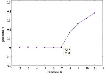
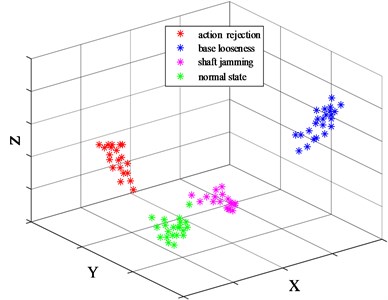
KFCM is used for clustering, the classification number $c$ is set to 4, and the three-dimensional spatial clustering results are shown in Fig. 9.

Fig. 9KFCM clustering results

The time-frequency joint feature vector matrix is sent to SVM for training. In order to improve the classification performance of SVM, the parameters of penalty factor C and mixing coefficient $\lambda$ are optimized according to the GWO algorithm proposed in document [10]. The number of iterations is set to 100, and the optimal parameter values are 2.5693 and 0.17 respectively.

Set the normal state sample eigenvalue label as 1 (1-20 groups), the shaft jamming as 2 (21-40 groups), the base looseness as 3 (41-60 groups), and the action rejection as 4 (61-80 groups). The identification results are as follows.

Fig. 10KFCM-SVM diagnosis results

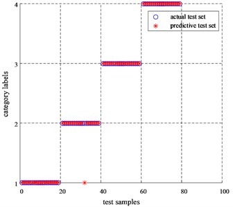
As can be seen from Fig. 10, except for one test sample of label 2, which was misclassified, all the other samples were classified correctly, and the identification result reached 98.75 %. Therefore, the model can accurately characterize the type of circuit breaker defect.

6.3. Comparative analysis of time-frequency joint features

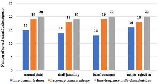
In order to compare the identification effects of single time-domain features, frequence-domain features and time-frequency multi-features, for the sample data in Section 5.1, KFCM-SVM is used for fault diagnosis, and the results are shown in Fig. 11.

The diagnostic accuracy rates of time-domain features and frequency-domain spectral entropy features were 72.5 % and 92.5 %, respectively, while the diagnostic accuracy of time-frequency multi-characteristics reached 98.75 %. It can be seen that the time-frequency characteristics can reflect the state information of the circuit breaker from multiple dimensions, the complementary feature is better than the single time or frequency features, and has good diagnostic performance.

Fig. 11Comparison of diagnosis results of time-frequency features

7. Conclusions

Accurately discriminating the operating state of circuit breakers using acoustic signals has always been a technical problem in fault diagnosis of electrical equipment. In this paper, through effective signal preprocessing and extraction of time-frequency joint features, accurate identification of circuit breaker states can be achieved:

1) A denoising method of background noise library combined with AWT is proposed, which effectively solves the problem of noise interference and provides a strong guarantee for accurate fault diagnosis.

2) A new multi-characteristics extraction method based on time-frequency combination is proposed, which can accurately characterize the state information of circuit breakers by extracting time-domain features and spectral difference entropy features of IMF components in frequency-domain from acoustic signals.

3) Based on the KFCM-SVM diagnostic model, this paper uses KFCM to pre-classify the samples, and then uses SVM for fault diagnosis, which can effectively improve the accuracy of circuit breaker fault diagnosis.