Abstract
As the core and precision component of a mechanical system, rolling element bearings would cause irreparable results once it breaks down. In order to study the dynamic response of bearing system caused by different localized defect sizes on outer raceway, a two-dimensional (2-D) explicit dynamics Finite Element Method (FEM) model of shaft-bearing-pedestal system with a localized defect is proposed. The model is verified by the experimental results. A new numerical method is used to investigate the influence of different defect sizes on the contact characteristics in this model. The indicator is introduced to study the contact force with different defect sizes. The results show that the increases with the increasing of defect depth and width, and the mathematic relationships are given for . Therefore, the dynamic FEM model can be used to bearing fault diagnosis and defect prediction.
Highlights
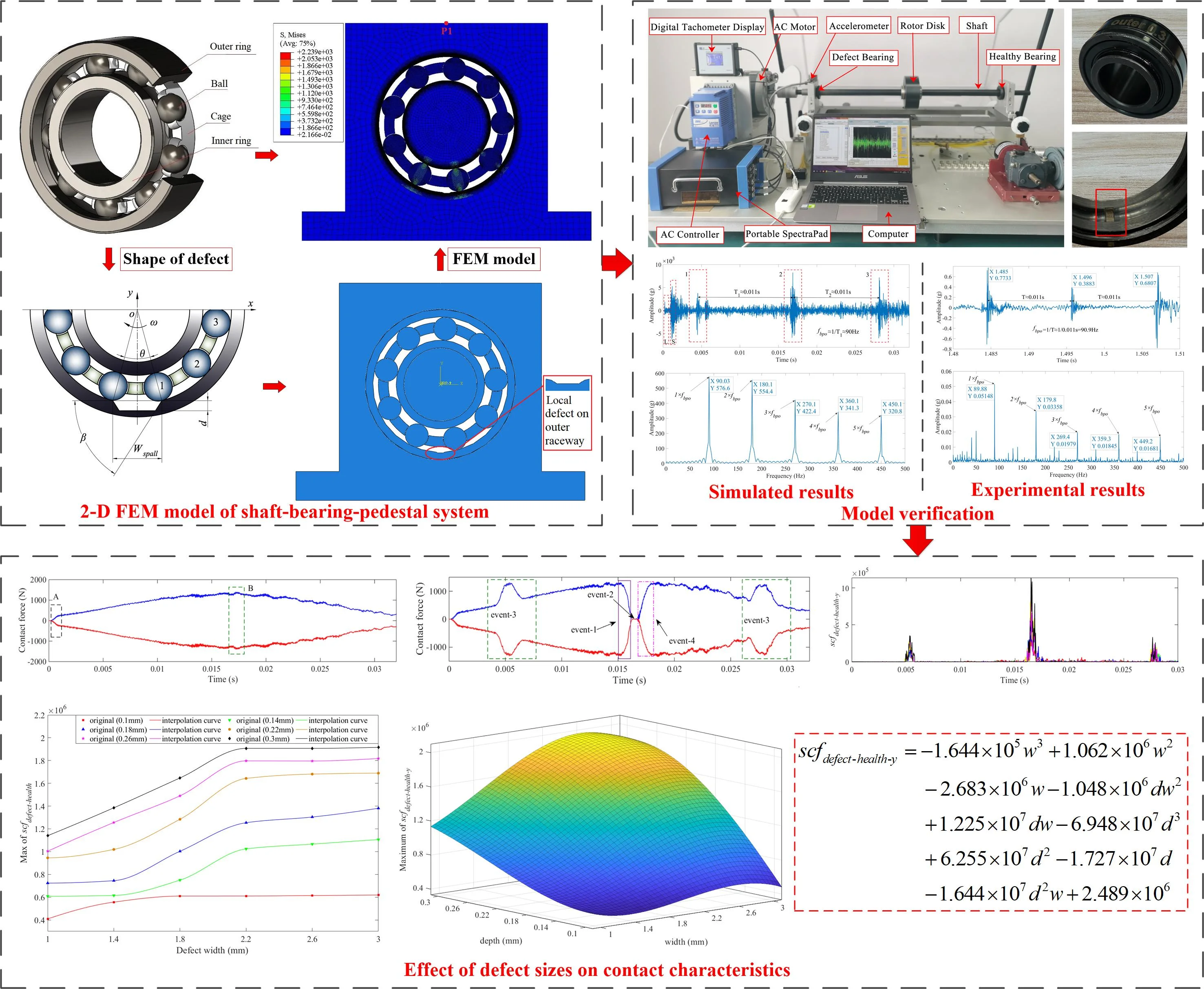
- A two-dimensional explicit dynamics Finite Element Method model of shaft-bearing-pedestal system with a localized defect on outer raceway surface is developed to investigate the influence of different defect sizes on the contact characteristics.
- The characteristics of the contact force for healthy and defective bearing are analyzed.
- The relationships between contact force and localized defect sizes are studied by the proposed indicator.
1. Introduction
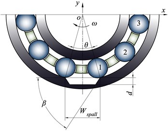
As one of the most significant parts of the machine, rolling element bearing is widely used in rotating machinery across various industries such as aerospace, railways, and renewable energy, etc. The damage or defects of rolling element bearings contribute to machinery breakdown, and consequently causing serious economic losses and even catastrophes in certain situations, such as air crash, rocket launch failure, train derailment and wind turbine shutdown, etc. [1-3]. Previous studies have shown that, when the localized defects (pits or spalls) appear on the raceway surface of rolling element bearing, a dual-impulse phenomenon would occur in the vibration signals [4-6], and a multi-event process would be shown with a rolling element pass over a defect. It includes the rolling element entering the defect, impacting the defect bottom, exiting from the defect, and the load compensation [7].
The models of rolling element bearing with localized defect were established to study dynamic response and contact characteristics [1-2, 8-9]. In general, these dynamic modeling methods for the bearing with local defect mainly include the analytical method and the Finite Element Method (FEM). Considering the effect of defect edge shape on bearing’s dynamic response, Liu et al. [10] established a dynamic model to investigate the vibration response of a ball bearing by utilizing the analytical method. Then, a 2 degree-of-freedom dynamic model of a cylindrical roller bearing with a localized surface defect was built to predict vibration response, in which effects of the radial load, defect sizes and types on the contact deformation and contact force between the roller and raceway are investigated [11]. Utilizing analytical method, Liu et al. studied the effects of dent [12], offset and bias local defects [13] on the outer raceway surface on dynamic response. In addition, Yang et al. [14] presented a dynamic analytical model of rotor-bearing-casing system to investigate the performance of the bearing defects and their transmission characteristics. Sawalhi et al. [15] proposed an analytical model of nonlinear multi-body dynamics to study the vibration response of rolling element bearing with localized defects, and found the dual-impulse in the experimental vibration signals. Luo et al. [16] built a coupled nonlinear dynamic model of the rolling element bearing with a spall on the inner raceway to analyze the dual-impulse time spacing by the transient collision force excited by the strike of the rolling element on the trailing edge of the spalled area.
Unfortunately, when the model of rolling bearing is established by the analytic method, several assumptions are introduced to simplify the model, such as neglecting the cage, mass of rolling elements, and roller slip, etc., which would affect the authenticity of the model to some extent. However, these assumptions are little considered in the FEM model, which can clearly reflect the operation of bearings. For example, the vibration response of defective bearing [17, 18] and degradation of high loaded oscillating bearings [19] were investigated by establishing the FEM model. Gradually, more detailed FEM models were constructed to simulate actual working conditions. Considering the mass of shaft, race, ball, and cage, a dynamic FEM model was developed by Shah and Patel [20] to predict the vibration generated by a healthy or localized defective deep groove ball bearing. When the factors such as material properties, friction coefficient and structural damping are taken into account, the vibration signals obtained by the FEM model is closer to those collected in actual working condition. Shao et al. [21] built a dynamic model by LS-DYNA, the deep groove ball bearing with fault on outer raceway was chosen to analyze the magnitude of the acceleration. Then, the influences of different localized defect shapes (square, hexagon, or circle) on the vibration response were studied [22]. Whereas, some factors were neglected in these FEM models of rolling element bearings mentioned above, such as the structural damping of bearings, the influences of pedestal and shaft on the vibration response of bearings, etc. It would lead to a large gap between the model and reality.
The appearance of the spall in rolling element bearing does not mean the end of the useful life. It is a more interesting and meaningful issue to replace the faulty bearing since a premature removal of the bearing from service may be very expensive, whereas suitable chances can be taken with the safety of machines and/or personnel [6]. Consequently, the study of defect evolution and the relationship between vibration signals of system response and defect size plays a significant role in prognostics and Product Health Management (PHM) of bearings. El-Thalji et al. [23-25] built a dynamic model of wear evolution to simulate the dynamic impact by utilizing multiple force diagrams, and obtained the transition points among the wear evolution stages by combining several models of contact mechanics, and explained the physical phenomena behind the detected signals from evolution dynamic model.
At present, the efforts on the relationship between system response and defect size mainly have been made on the influence of bearing load, contact angle and defect prediction. In order to study the effects of defect size on load distributions, Xu et al. [26] developed a model of angular contact ball bearing with a local defect on outer raceway. Mouloud et al. [27] proposed a new method based on Full Factorial Design (FFD) for the prediction of the size of the spalls on the contact surfaces of thrust ball bearings, and analyzed the effect of the factors such as rotational speed, load, spalling size, the position of the sensors, frequency range on the vibrations level, and the interaction between them. Liu et al. [28] presented a FEM model to study the effects of the horizontal and slant subsurface cracks on the contact characteristics in a roller bearing, and obtained the mathematic relationship between the contact characteristics and crack sizes by using a polynomial fitting approach. Considering the surface crack, Shi et al. [29] proposed a dynamic model of the roller bearing to study the influences of the surface crack sizes (depth and slope angle) on the bearing vibration and contact characteristics.
These researches on the relationship between the system response and defect size are mainly based on the vibration signals of bearing rather than the contact characteristics, which can more directly reflect the contact and operation state of the bearing. In addition, it is shown from their results that the size of spalling defect is only related to the contact force between the rolling element and the raceway, but does not indicate the influence of defect depth. In order to study the relationship between contact characteristics and defect size, considering the influence of pedestal and shaft on the dynamic characteristics, a 2-D explicit dynamics FEM model of rolling element bearing with a localized defect is established in this paper. The FEM model is verified by experimental results. Taking the depth and width of defect into account, the operation process of rolling element bearing with a local defect is simulated. The relationships between contact force and localized defect sizes on the outer raceway are analyzed.
The rest of this paper is organized as follows: in Section 2, a 2-D explicit dynamics FEM model of shaft-bearing-pedestal system with a localized defect on the outer raceway of deep groove ball bearing ER-16k is established. In Section 3, both the time-domain and frequency-domain vibration signals of the FEM model are analyzed. The FEM model is verified by the experimental results collected from the Machinery Fault Simulator (MFS) test rig in Section 4. In Section 5, the multi-event process of contact force is described and the effects of defect sizes on contact force are discussed. Some conclusions have been drawn in Section 6.
2. Construction of model
Taking the deep groove ball bearing ER-16k shown in Fig. 1, a comprehensive shaft-bearing-pedestal system model would be established, which is shown in Fig. 2, and its dimensions of parameters are shown in Table 1. It is noted that the clearance between the cage pocket and the rolling element is 0.3 mm.
Fig. 1Deep groove ball bearing ER-16k
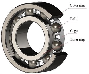
Fig. 2Shaft-bearing-pedestal system
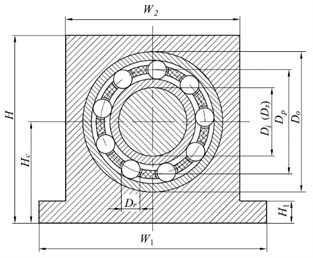
Table 1Dimensions of parameters
Parameter | |||||||||||
Value (mm) | 52 | 25.4 | 40.7 | 38.7 | 8 | 25.4 | 90 | 45.35 | 12 | 110 | 70 |
2.1. 2-D FEM model of shaft-bearing-pedestal system
In order to build FEM model of the shaft-bearing-pedestal system conveniently, these simplifications and assumptions are given as follows:
(1) The chamfers on the inner and outer rings, shaft and pedestal have slight effect on the dynamic response of the bearing, only are important for assembly process, therefore these chamfers are ignored.
(2) The threaded holes on the pedestal are ignored.
(3) Since the temperature of bearing is almost constant in a short simulation time, thermal effect of the model can be ignored.
(4) Because deep groove ball bearing ER-16k is usually applied radial load, the influences of axial load would be neglected in this model.
(5) It is assumed that all components are isotropic materials.
Based on the simplifications mentioned above, a 2-D FEM model of shaft-bearing-pedestal system is built as shown in Fig. 3. The morphology characteristics of the defect is shown in Fig. 4, which is located at the 6 o'clock position on the outer raceway. The defect angle is 45° and the defect size (width × depth) is 3 mm×0.3 mm.
Fig. 32-D FEM model
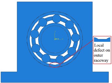
Fig. 4Morphology characteristics of defect
2.2. Material properties
In this FEM model, all types of components are regarded as deformable. The rings and rolling elements are made of GCr15. The materials of cage, bearing pedestal and the shaft are nylon, HT150 and 40Cr, respectively. The properties of the materials are shown in Table 2.
Table 2Material properties
Young’s modulus (GPa) | Poisson’s ratio | Structural damping’s ratio | Density (kg/m3) | |
GCr15 | 219 | 0.3 | 0.01 | 7850 |
Nylon | 28.3 | 0.4 | 0.13 | 1350 |
HT150 | 116 | 0.19 | 0.02 | 7150 |
40Cr | 206 | 0.29 | 0.01 | 7820 |
2.3. Loads and boundary conditions
There are three sequential explicit dynamic steps. The first one is named loading step (0.001 s), which is used to exerted the force. The second one is named speed step (0.001 s), which is used to apply the speed of inner ring. The last one is named propagated step (0.030 s), which would maintain the previous force and speed applied on the model in the subsequent simulation time. The sampling frequency is 100 kHz.
In general, bearing dynamics are very complicated with interactions among the rolling elements, cage, and raceways. Therefore, the loads and boundary conditions below are given to simulate the running of bearing under typical operating conditions in the FEM model:
(1) The gravitational acceleration of 9.8 m/s2 is applied to the system.
(2) A radial load of 25 N on the center of the shaft in the negative global -direction is applied.
(3) The cage is created as nine discrete parts, which are constrained as a whole by coupling constraints. The rotational speed is not applied to the outer ring and inner ring directly, the inner ring will rotate with the rotating shaft. The shaft rotates at 1500 r/min in a clockwise direction.
2.4. Discretization of FEM model
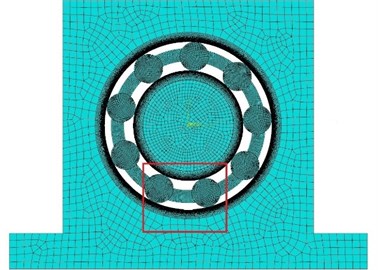
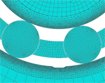
Mesh is an important step for discretization of FEM model. In order to obtain high quality elements, the rolling elements are meshed with mixture of quadrilateral and triangular elements (qua-dominated). The appropriate element size is critical for analysis accuracy and time in FEM model simulation. Because the vibration of bearing is mainly caused by interactions between rolling elements and raceways, the surfaces of the inner and outer raceway are meshed by the smaller element size 0.1 mm. The element size 0.5 mm is chosen to mesh the rolling elements, cage and other zones of inner and outer rings. The element sizes of pedestal and shaft are chosen as 1 mm. The mesh of the FEM model is shown in Fig. 5.
Fig. 5Images of meshed model: a) whole meshed model, b) enlarged meshed part in red zone
a)
b)
3. Analysis of simulation results
3.1. Results and analysis of simulated signals in time domain
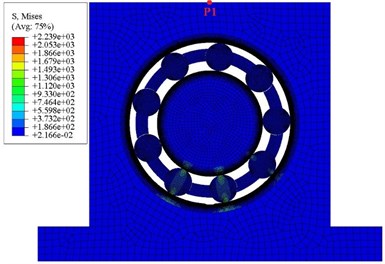
The FEM model of bearing with localized defect is established and simulated, the stress contour of the FEM model is shown in Fig. 6. There are three rolling elements in the loading zone of the bearing. It is worthy to note that the stress field near the contact surface between outer ring and pedestal is non-zero when the rolling element passes over the loading zone. Because a rigid pedestal would enhance the stiffness of FEM model, and result in an unrealistic increase in the amplitude of vibration signals, it is more suitable to define pedestal as a deformable rather than a rigid body in FEM modeling. The vibration acceleration signals of the bearing are sampled from point P1 shown as Fig. 6 for analysis.
Fig. 6Stress contour
It is shown in Fig. 7 that the acceleration signals of vibration in time domain. When the loading and speed of the bearing are applied during 0-0.002 s, which would excite the first and second pulses, marked as L and S in the red dotted boxes, respectively. While the rolling elements 1, 2 and 3 pass through the defect, the three dual-impulse signals would be excited sequentially. Therefore, the FEM model is reasonable by analysis of the acceleration signals of vibration in the time domain.
Fig. 7Simulated acceleration signals of vibration in time domain
3.2. Analysis of simulated signals in frequency domain
The frequency spectrum of acceleration signals obtained by FFT is shown in Fig. 8, and the characteristic frequency of the outer raceway () and its harmonic frequencies are obvious. The can be calculated by Eq. (1):
where, is the rotation frequency of the shaft, describes the number of balls, denotes the ball diameter, refers to the bearing pitch diameter, and represents the contact angle.
Fig. 8Frequency spectrum of FEM model
The parameters of bearing ER-16k related to the Eq. (1) are given in Table 1 and contact angle . According to Eq. (1), the theoretical is 89.24 Hz. The of simulated signals is 90.03 Hz. The FEM simulated fits the theoretical very well. The difference between them is 0.88 %, Therefore, the FEM model is reliable and can be used to analyze the response of vibration and contact characteristics in further.
4. Experiment verification
In order to verify the FEM model, an experiment based on the MFS test rig is conducted on a bearing with a localized defect on outer raceway. In the experiment, the inner ring of the bearing is applied with a radial load of 25 N under 1500 r/min.
4.1. Experimental test rig
The MFS test rig produced by Spectra Quest Incorporation (SQI) in USA is used to test the localized defect on outer raceway surface of bearing, which is shown in Fig. 9.
Fig. 9MFS test rig
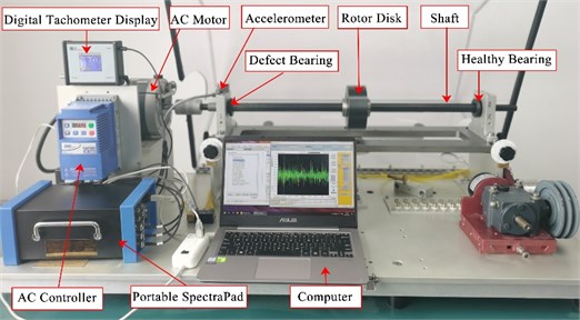
In this experiment, the shaft was driven by a 1 HP 3-phase AC motor at 1500 r/min. The motor was connected with shaft by a flexible coupling. The shaft was supported by two deep groove ball bearings ER-16k, one is localized defect bearing and the other is healthy bearing. An ICP tri-axial accelerometer is mounted on top of the pedestal of the defective bearing to sample the acceleration signals of vibration. A 50 N radial load was put on the shaft by a 5.1 kg rotor disk installed in the middle of the two bearings, therefore each bearing supports a 25 N radial load. The AC controller was used to control the start and stop of the motor, set the speed of the motor and the safety protection of the system, the digital tachometer display was used to show the actual speed of the motor. A DAQ acquisition card of portable spectra PAD connected between the accelerometer by a 3-channel data cable and a computer by USB port, was used to collect acceleration signals of vibration, which limit sampling frequency is 102.4 kHz. After AC motor was running stable, three groups of the acceleration signals of vibration were collected with a sampling frequency of 66 kHz, and the duration was 4 s.
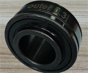
It is shown as Fig. 10, the bearing with localized defect was installed near the motor, which parameters are width 3 mm, depth 0.3 mm and defect angle 90°.
Fig. 10Experimental bearing, a) defective bearing ER-16k, b) fabricated defect on outer raceway
a)
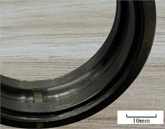
b)
4.2. Model verification by experimental results
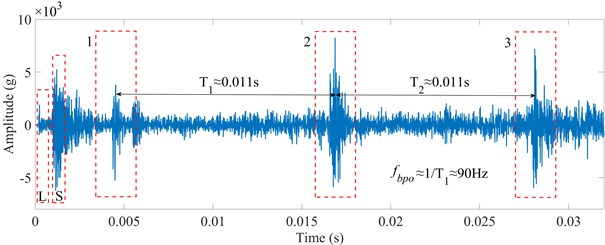
One group of signals is randomly selected from the three groups of acceleration signals of vibration collected from the test rig to verify FEM model, which is shown in Fig. 11(a). The acceleration signals of vibration during 1.3 to 1.6 s are taken to analyze the faulty information, as shown in Fig. 11(b). Furthermore, it is shown in Fig. 11(c) that the acceleration signals of vibration in 1.48 to 1.51 s are enlarged. It is obvious that the dual-impulse are excited while the rolling element passing across the defect, and the time interval between two dual-impulse approximates 0.011 s, which fits with the result of FEM model as shown in Fig. 7.
Fig. 11Experimental acceleration signals of vibration, a) 0-4 s, b) 1.3-1.6 s, c) 1.48-1.51 s
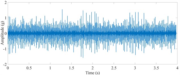
a)
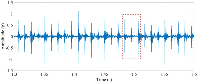
b)
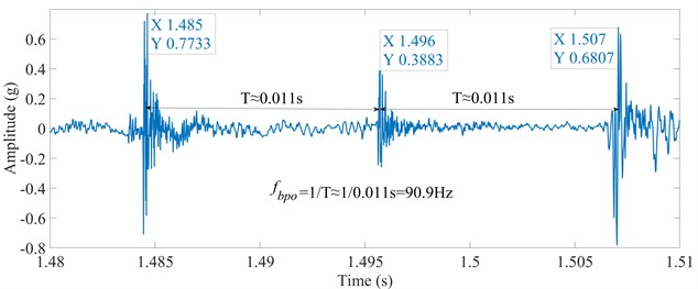
c)
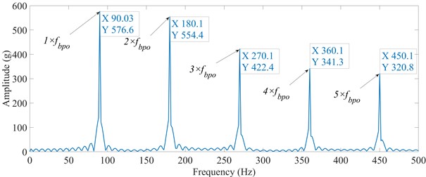
Fig. 12Frequency spectrum of experimental acceleration signals
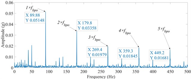
The frequency spectrum of experimental acceleration signals is obtained by FFT, as shown in Fig. 12. The characteristic frequency and its harmonic frequency can be clearly found. It is obvious that the of experimental results is 89.88 Hz, while the of the simulated results is 90.03 Hz. The difference between the results of the experiment and simulation is only 0.2 %, which is almost consistent. The small difference of between simulation and experiment comes from the slight difference between the actual speed and the set speed of the motor in the experiment. Therefore, the FEM model is almost accurate and the data from the FEM model could be analyzed through other methods to get more information.
5. Effect of defect sizes on contact characteristics
5.1. Contact force and multi-event process
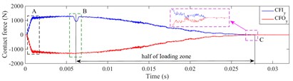
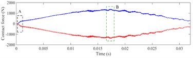
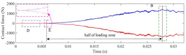
As shown in Fig. 4, the three rolling elements on the right side of the 6 o'clock of bearing are marked as ball 1, ball 2 and ball 3 counterclockwise. The contact forces between these rolling elements and the inner and outer raceway are extracted from the FEM models of a healthy bearing and a defective bearing, respectively. The defect angle 45° and size is 3 mm×0.3 mm. The contact forces between the rolling elements and the outer raceway in the -direction and -direction are represented as and , respectively. Similarly, the contact forces between the rolling elements and the inner raceway are expressed as and , respectively.
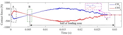
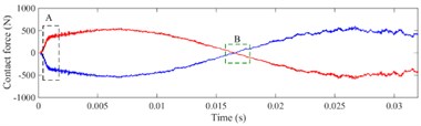
The contact force and of healthy bearing in the -direction and -direction are shown as Fig. 13 and Fig. 14, respectively. The curve in the black box 'A' is the loading process of the simulation. The green box 'B' is the position where the rolling element runs to the 6 o'clock of the bearing, which is the center of the load zone. The boxes 'E' and 'C' are the start and end points of load zone, respectively.
Fig. 13Contact force of healthy bearing in x-direction, a) ball 1, b) ball 2, c) ball 3
a)
b)
c)
Fig. 14Contact force of healthy bearing in y-direction, a) ball 1, b) ball 2, c) ball 3
a)
b)
c)
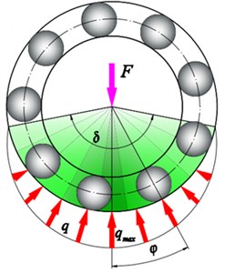
The contact characteristics of the bearing could be clearly reflected by contact force between the rolling elements and raceway in the running process. The loading zone of bearing is shown in Fig. 15, it is visually shown that rolling elements are entering or exiting the load zone, the range of the load zone, and the time from the rolling element running to the bottom of the load zone. When the bearing starts to rotate, the of ball 1 appears a rapid increase, which is the loading process (box 'A' in Fig. 13).
Ball 1 is at the lower left side of the outer raceway, which is located at the load zone. The will increase sharply, while the bearing starts running and loading. Then, the and of ball 1 decrease at the same time and finally intersect on the zero lines, because ball 1 has reached the 6 o'clock of the outer ring (box 'B' in Fig. 13), the component force of the contact force in the -direction is zero, all concentrated in the y-direction ( and have been kept above 1000 N in this period), as shown in Fig. 14. With the rotation of the inner ring, ball 1 gradually exits from the load zone, and the contact force between ball 1 and raceways gradually reduces to zero. Ball 1 exits the load zone when , , and decrease to zero at the same time. The time interval from ball arriving at the bottom of raceway to exiting the load zone is half of the time when ball passes the load zone. Since the load zone can be calculated by Eqs. (2) and (3):
where is the arc length of load zone, is the center angle of load zone, is the time from roller running to the bottom of the raceway to exiting point of the load zone, is the angular speed of inner raceway, is the diameter of outer raceway.
Fig. 15Load zone of bearing
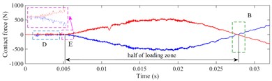
Noteworthy, it is shown in Fig. 13(c) and Fig. 14(c), that the , , and are zero in theory, because the ball 3 is not located at the load zone before the box 'E'. However, the , in zone 'D' shown as Fig. 13(c) present a series of small pulses during some times. Before ball 3 enters into the load zone, it is located near the -direction. Since the centrifugal force of ball 3 would cause slight impacts, the contact force caused by these impact acts on the horizontal direction (-direction), the component of the contact force in the vertical direction (-direction) is 0.
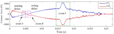
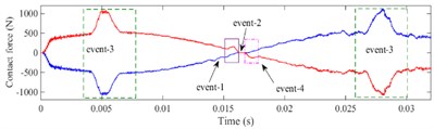
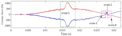
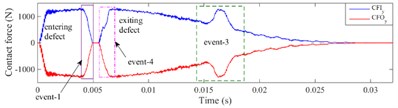
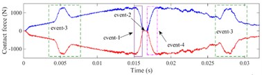
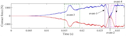
The contact force and of defective bearing in the -direction and -direction are shown in Fig. 16 and Fig. 17, respectively. When rolling element enters or exits the defect, it is obvious that the contact force between the rolling element and the inner, outer raceway presents a multi-event process [23]. Taking ball 1 passing through the defect as an example, the multi-event process is described as following.
At the beginning of applying load, the absolute value of the contact force in and directions between ball 1 and raceway would increase, which are shown in Fig. 16(a) and Fig. 17(a), respectively. During the stage of applying speed, because ball 1 moves near the 6 o'clock of the outer ring, the contact force is mainly in the vertical component at this time, which leads to the being a downward trend and the being a slow-increasing trend. At 0.004 s, ball 1 runs to the edge of the defect, the reaches the maximum. As ball 1 enters the defect with the 45° slope, the , , and of ball 1 will decrease gradually. When ball 1 enters the defect completely, contact forces , , and would decrease to 0 because of the unloading of ball 1. The process of the rolling element entering the defect is regarded as “event-1”, which is shown in Fig. 16 and Fig. 17.
Fig. 16Contact force of defective bearing in x-direction, a) ball 1, b) ball 2, c) ball 3
a)
b)
c)
Fig. 17Contact force of defective bearing in y-direction, a) ball 1, b) ball 2, c) ball 3
a)
b)
c)
When ball 1 has entered the defect completely (0.005-0.006 s), this process is considered as event-2, as shown in “event-2” in Fig. 16 and Fig. 17. When the depth of the defect is small, ball 1 will impact on the bottom of the defect due to inertia force, which causes slight pulses on its contact force. But while the depth of the defect is large, the cage carries ball 1 in its pocket hole so that it does not approximately impact the bottom of the defect.
As the bearing rotates continuously, ball 1 begins to contact the defect edge and gradually exits the defect after 0.006 s. The contact forces in horizontal direction and increase, contrarily the contact force in vertical direction and increase rapidly to the maximum value in a short time. Since the defect is located on the outer raceway, ball 1 would impact the edge of the defect, then the bearing will reload, the increases faster than . The process of the rolling element exiting the defect and impacting with the edge of the defect is defined as “event-4”, which is shown in Fig. 16 and Fig. 17.
When ball 2 crosses over the defect, it will endure a process of load redistribution. As ball 2 is at the unloading stage, the original load supported by ball 2 will be shared by the other rolling elements within the load area, which causes the contact force of ball 1 and ball 3 to increase rapidly. As ball 2 is at the reloading stage, the contact force of ball 1 and ball 3 will decrease to the normal level. The process is called load compensation and is defined as “event-3”, which is shown in Fig. 16 and Fig. 17.
5.2. Effect of defect sizes on contact force
It is shown from the above studies that the amplitude trend of the contact force in the defective bearing is similar to that in the healthy bearing, except when the rolling elements pass over the defect. In order to investigate the influence of defect sizes on contact force, the indicator is constructed, which is as Eq. (4):
where, and are the contact force in the defective and healthy bearing, respectively.
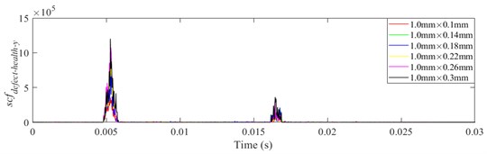
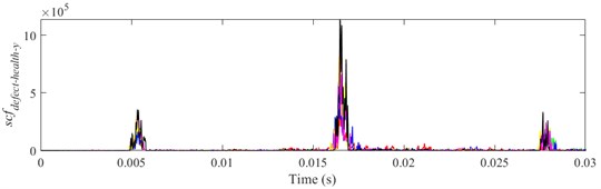
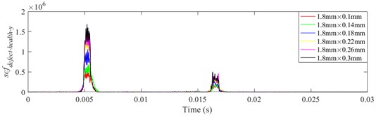
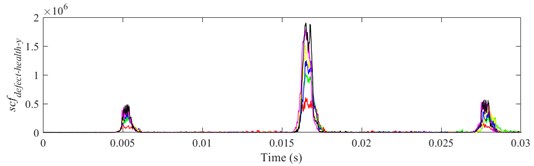
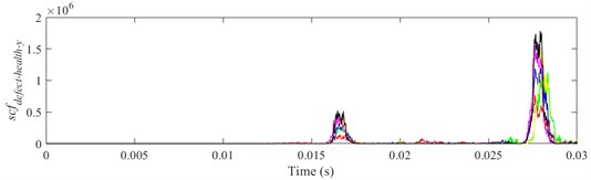
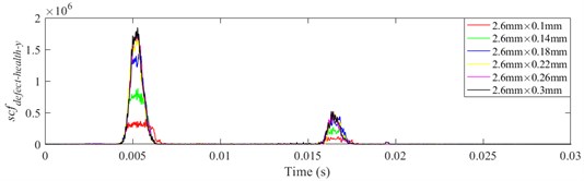
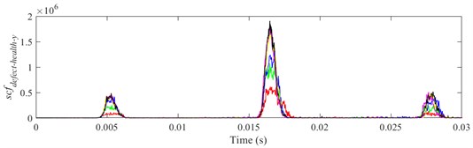
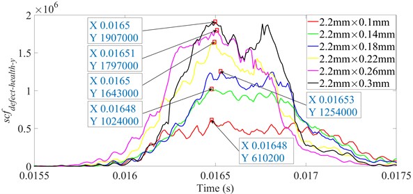
Since the defect is located in the 6 o'clock direction on outer raceway, the contact force between rolling elements and raceway is obviously shown in the -direction near the defect region. A series of cases with different defect width and depth listed in Table 3 are simulated to calculate by the contact force between rolling elements and outer raceway. The indicator in -direction between ball 1, 2, 3 and raceway corresponding to different defect widths 1.0, 1.4, 1.8, 2.2, 2.6 and 3.0 mm are shown in Figs. 18-23(a), (b) and (c), respectively.
Fig. 18scfdefect-health-y of different defect depths when defect width is 1.0 mm, a) ball 1, b) ball 2, c) ball 3
a)
b)
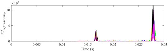
c)
Fig. 19scfdefect-health-y of different defect depths when defect width is 1.4 mm, a) ball 1, b) ball 2, c) ball 3
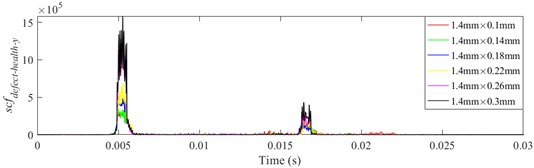
a)
b)
c)
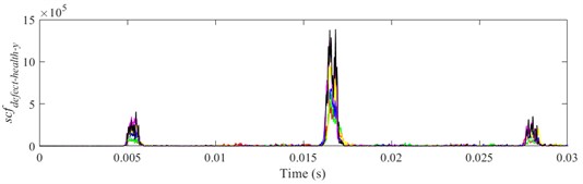
Fig. 20scfdefect-health-y of different defect depths when defect width is 1.8mm, a) ball 1, b) ball 2, c) ball 3
a)
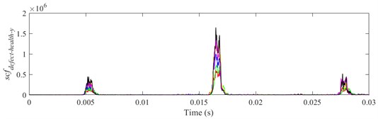
b)
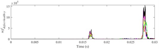
c)
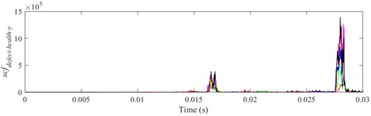
Fig. 21scfdefect-health-y of different defect depths when defect width is 2.2 mm, a) ball 1, b) ball 2, c) ball 3
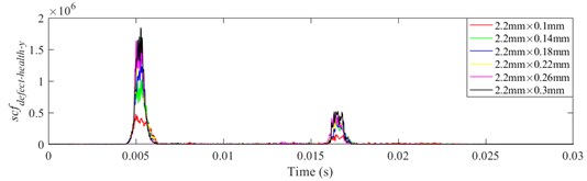
a)
b)
c)
Fig. 22scfdefect-health-y of different defect depths when defect width is 2.6 mm, a) ball 1, b) ball 2, c) ball 3
a)
b)
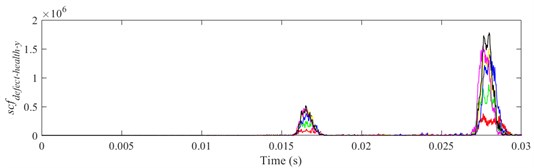
c)
Fig. 23scfdefect-health-y of different defect depths when defect width is 3.0 mm, a) ball 1, b) ball 2, c) ball 3
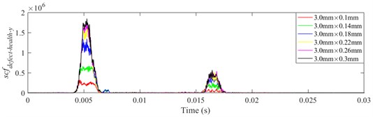
a)
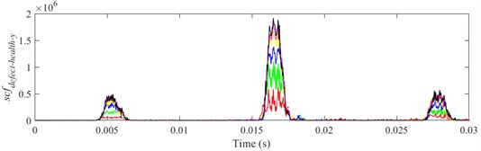
b)
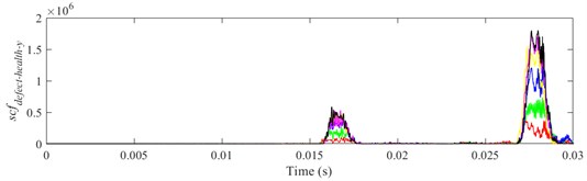
c)
Table 3Defect with different width and depth
Sizes | Width/mm | ||||||
1.0 | 1.4 | 1.8 | 2.2 | 2.6 | 3.0 | ||
Depth / mm | 0.1 | 1.0×0.1 | 1.4×0.1 | 1.8×0.1 | 2.2×0.1 | 2.6×0.1 | 3.0×0.1 |
0.14 | 1.0×0.14 | 1.4×0.14 | 1.8×0.14 | 2.2×0.14 | 2.6×0.14 | 3.0×0.14 | |
0.18 | 1.0×0.18 | 1.4×0.18 | 1.8×0.18 | 2.2×0.18 | 2.6×0.18 | 3.0×0.18 | |
0.22 | 1.0×0.22 | 1.4×0.22 | 1.8×0.22 | 2.2×0.22 | 2.6×0.22 | 3.0×0.22 | |
0.26 | 1.0×0.26 | 1.4×0.26 | 1.8×0.26 | 2.2×0.26 | 2.6×0.26 | 3.0×0.26 | |
0.3 | 1.0×0.3 | 1.4×0.3 | 1.8×0.3 | 2.2×0.3 | 2.6×0.3 | 3.0×0.3 | |
Fig. 24scfdefect-health-y between ball 2 and outer raceway during 0.0155-0.0175 s when defect width is 1.0 mm
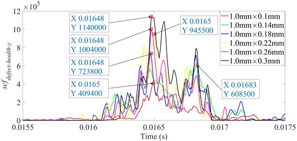
It is shown from Figs. 18-23 that the indicator would increase during event-2 and event-3, and is close to zero in the other periods. When and would be close to the maximum during event-2, the peak of indicator during event-2 is higher than that during event-3. Therefore, the indicator can reflect the difference of contact force between healthy bearing and defective bearing when ball enters defect. In order to study the peak of indicator further, Figs. 18-23(b) from 0.0155-0.0175 s are enlarged as Figs. 24-29, respectively.
Fig. 25scfdefect-health-y between ball 2 and outer raceway during 0.0155-0.0175 s when defect width is 1.4 mm
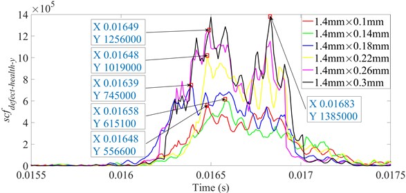
Fig. 26scfdefect-health-y between ball 2 and outer raceway during 0.0155-0.0175 s when defect width is 1.8 mm
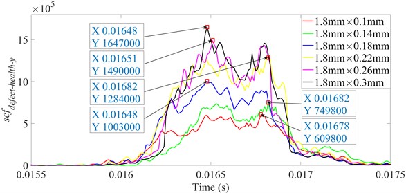
Fig. 27scfdefect-health-y between ball 2 and outer raceway during 0.0155-0.0175 s when defect width is 2.2 mm
In order to investigate the effect of defect sizes on the maximum of indicator , the maximum of indicator corresponding to different defect widths and depths are performed via cubic spline interpolations, which is shown in Fig. 30.
Fig. 28scfdefect-health-y between ball 2 and outer raceway during 0.0155-0.0175 s when defect width is 2.6 mm
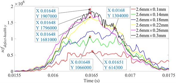
Fig. 29scfdefect-health-y between ball 2 and outer raceway during 0.0155-0.0175 s when defect width is 3.0 mm
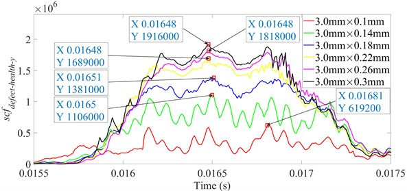
Fig. 30Cubic spline interpolation to maximum of indicator scfdefect-health-y when defect width is from 1.0 to 3.0 mm
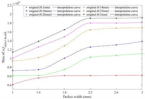
As shown in Fig. 30, when the defect depth is the same, maximum of indicator increases with the defect width increases. However, when the width of defect reaches a certain value, the indicator is close to the maximum value. When the defect width is small (1.0-2.2 mm), rolling elements would not impact the bottom of the defect as passing over the defect, therefore the contact force of rolling element bearings with different defect widths is quite different. With increasing of defect width (2.2-3.0 mm), rolling elements could completely collide with the bottom of defect when they pass through the defect, therefore the maximum of indicator would not change significantly.
When the defect width is the same, the maximum values of indicator would be higher with deeper defect during ball 2 passing through the defect. When the defect depth is small, the rolling element would not unload completely as entering the defect, therefore contact force of defective bearing grows gradually. Distinctively, the maximum value of indicator in red is defect depth being 0.1 mm with different defect widths. It would reach the maximum value very quickly, because when the defect depth is small, a slight increase with the defect width would lead to the rolling element impacting the bottom of defect, at which stage the contact force does not change significantly even if the defect widens further.
Fig. 31Effects of defect sizes on maximum of indicator scfdefect-health-y
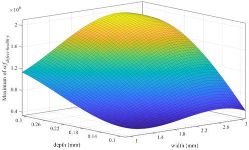
Fig. 31 shows the effects of the defect width and depth on the maximum of indicator . Here, the defect width are 1.0, 1.4, 1.8, 2.2, 2.6 and 3.0 mm; the defect depth are 0.1, 0.14, 0.18, 0.22, 0.26 and 0.3 mm, respectively. A polynomial fitting approach is applied to obtain the mathematic relationship between the maximum of indicator and defect sizes. According to the simulation results in Fig. 31, the relationship between the maximum of indicator and defect sizes is given as:
where, is the defect width, is the defect depth.
According to the above analysis, the contact force between rolling elements and raceways could be greatly affected by the defect sizes. The established approach can give a useful numerical method for analyzing the contact characteristics of a rolling element bearing with localized defect, and provide innovative theoretical guidance for bearing fault diagnosis and defect prediction.
6. Conclusions
The localized defect evolution process of rolling element bearing is simulated by FEM model. The following conclusions can be drawn:
1) Considering the structural damping of the bearing and the sliding of the rolling element, a 2-D explicit dynamics FEM model including the bearing with localized defects, shaft-bearing-pedestal is established. An experiment based on the Machinery Fault Simulator test rig is performed to verify the applicability of the FEM model.
2) The contact force between rolling elements and raceways both in and directions are discussed separately for healthy and defective bearing, the multi-event process of contact force is described. The comparison results show that the amplitude trend of the contact force in the defective bearing is similar to that in the healthy bearing, except when the rolling elements pass over the defect.
3) A novel indicator is constructed and the maximum of indicator corresponding to different defect widths and depths are analyzed. A polynomial fitting approach is applied to obtain the mathematic relationship between the maximum of indicator and defect sizes, which can investigate the contact characteristics of a rolling element bearing with the localized defect.
References
-
S. Singh, C. Q. Howard, and C. H. Hansen, “An extensive review of vibration modelling of rolling element bearings with localised and extended defects,” Journal of Sound and Vibration, Vol. 357, pp. 300–330, Nov. 2015, https://doi.org/10.1016/j.jsv.2015.04.037
-
J. Liu and Y. Shao, “Overview of dynamic modelling and analysis of rolling element bearings with localized and distributed faults,” Nonlinear Dynamics, Vol. 93, No. 4, pp. 1765–1798, Sep. 2018, https://doi.org/10.1007/s11071-018-4314-y
-
Z. Zhao, X. Yin, and W. Wang, “Effect of the raceway defects on the nonlinear dynamic behavior of rolling bearing,” Journal of Mechanical Science and Technology, Vol. 33, No. 6, pp. 2511–2525, Jun. 2019, https://doi.org/10.1007/s12206-019-0501-0
-
N. Sawalhi and R. B. Randall, “Vibration response of spalled rolling element bearings: observations, simulations and signal processing techniques to track the spall size,” Mechanical Systems and Signal Processing, Vol. 25, No. 3, pp. 846–870, Apr. 2011, https://doi.org/10.1016/j.ymssp.2010.09.009
-
A. Moazen Ahmadi, D. Petersen, and C. Howard, “A nonlinear dynamic vibration model of defective bearings – The importance of modelling the finite size of rolling elements,” Mechanical Systems and Signal Processing, Vol. 52-53, No. 1, pp. 309–326, Feb. 2015, https://doi.org/10.1016/j.ymssp.2014.06.006
-
A.-B. Ming, W. Zhang, Z.-Y. Qin, and F.-L. Chu, “Dual-impulse response model for the acoustic emission produced by a spall and the size evaluation in rolling element bearings,” IEEE Transactions on Industrial Electronics, Vol. 62, No. 10, pp. 6606–6615, Oct. 2015, https://doi.org/10.1109/tie.2015.2463767
-
B. Q. Chang et al., “Dynamic modeling for rolling bearings under multi-event excitation,” (in Chinese), Journal of Vibration and Shock, Vol. 37, No. 17, pp. 16–24, 2018.
-
S.-W. Hong and V.-C. Tong, “Rolling-element bearing modeling: A review,” International Journal of Precision Engineering and Manufacturing, Vol. 17, No. 12, pp. 1729–1749, Dec. 2016, https://doi.org/10.1007/s12541-016-0200-z
-
A. Kumar and R. Kumar, “Role of signal processing, modeling and decision making in the diagnosis of rolling element bearing defect: A review,” Journal of Nondestructive Evaluation, Vol. 38, No. 1, pp. 1–29, Mar. 2019, https://doi.org/10.1007/s10921-018-0543-8
-
J. Liu and Y. Shao, “A new dynamic model for vibration analysis of a ball bearing due to a localized surface defect considering edge topographies,” Nonlinear Dynamics, Vol. 79, No. 2, pp. 1329–1351, Jan. 2015, https://doi.org/10.1007/s11071-014-1745-y
-
J. Liu, Z. Shi, and Y. Shao, “An analytical model to predict vibrations of a cylindrical roller bearing with a localized surface defect,” Nonlinear Dynamics, Vol. 89, No. 3, pp. 2085–2102, Aug. 2017, https://doi.org/10.1007/s11071-017-3571-5
-
J. Liu, Z. Xu, Y. Xu, X. Liang, and R. Pang, “An analytical method for dynamic analysis of a ball bearing with offset and bias local defects in the outer race,” Journal of Sound and Vibration, Vol. 461, p. 114919, Nov. 2019, https://doi.org/10.1016/j.jsv.2019.114919
-
J. Liu, H. Wu, and Y. Shao, “A theoretical study on vibrations of a ball bearing caused by a dent on the races,” Engineering Failure Analysis, Vol. 83, pp. 220–229, Jan. 2018, https://doi.org/10.1016/j.engfailanal.2017.10.006
-
Y. Z. Yang, W. Z. Wang, and D. X. Jiang, “Simulation and experimental analysis of rolling element bearing fault in rotor-bearing-casing system,” Engineering Failure Analysis, Vol. 92, pp. 205–221, 2018, https://doi.org/10.1016/j.engfailanal
-
N. Sawalhi and R. B. Randall, “Simulating gear and bearing interactions in the presence of faults,” Mechanical Systems and Signal Processing, Vol. 22, No. 8, pp. 1952–1966, Nov. 2008, https://doi.org/10.1016/j.ymssp.2007.12.002
-
M. Luo, Y. Guo, H. Andre, X. Wu, and J. Na, “Dynamic modeling and quantitative diagnosis for dual-impulse behavior of rolling element bearing with a spall on inner race,” Mechanical Systems and Signal Processing, Vol. 158, No. 7, p. 107711, Sep. 2021, https://doi.org/10.1016/j.ymssp.2021.107711
-
T. Slack and F. Sadeghi, “Explicit finite element modeling of subsurface initiated spalling in rolling contacts,” Tribology International, Vol. 43, No. 9, pp. 1693–1702, Sep. 2010, https://doi.org/10.1016/j.triboint.2010.03.019
-
A. Nabhan, M. Nouby, A. Sami, and M. Mousa, “Vibration analysis of deep groove ball bearing with outer race defect using ABAQUS,” Journal of Low Frequency Noise, Vibration and Active Control, Vol. 35, No. 4, pp. 312–325, Dec. 2016, https://doi.org/10.1177/0263092316676414
-
F. Massi et al., “Degradation of high loaded oscillating bearings: Numerical analysis and comparison with experimental observations,” Wear, Vol. 317, pp. 141–152, 2014, https://doi.org/10.1016/j.wear
-
D. S. Shah and V. N. Patel, “A dynamic model for vibration studies of dry and lubricated deep groove ball bearings considering local defects on races,” Measurement, Vol. 137, pp. 535–555, Apr. 2019, https://doi.org/10.1016/j.measurement.2019.01.097
-
Y. Shao, W. Tu, and F. Gu, “A simulation study of defects in a rolling element bearing using FEA,” in 2010 International Conference on Control, Automation and Systems (ICCAS 2010), pp. 596–599, Oct. 2010, https://doi.org/10.1109/iccas.2010.5669813
-
J. Liu, Y. Shao, and M. J. Zuo, “The effects of the shape of localized defect in ball bearings on the vibration waveform,” Proceedings of the Institution of Mechanical Engineers, Part K: Journal of Multi-body Dynamics, Vol. 227, No. 3, pp. 261–274, Sep. 2013, https://doi.org/10.1177/1464419313486102
-
I. El-Thalji and E. Jantunen, “Dynamic modelling of wear evolution in rolling bearings,” Tribology International, Vol. 84, pp. 90–99, Apr. 2015, https://doi.org/10.1016/j.triboint.2014.11.021
-
I. El-Thalji and E. Jantunen, “Fault analysis of the wear fault development in rolling bearings,” Engineering Failure Analysis, Vol. 57, pp. 470–482, Nov. 2015, https://doi.org/10.1016/j.engfailanal.2015.08.013
-
I. El-Thalji and E. Jantunen, “A descriptive model of wear evolution in rolling bearings,” Engineering Failure Analysis, Vol. 45, pp. 204–224, Oct. 2014, https://doi.org/10.1016/j.engfailanal.2014.06.004
-
X. Li et al., “Analysis of varying contact angles and load distributions in defective angular contact ball bearing,” Engineering Failure Analysis, Vol. 91, pp. 449–464, Sep. 2018, https://doi.org/10.1016/j.engfailanal.2018.04.050
-
M. Boumahdi, S. Rechak, and S. Hanini, “Analysis and prediction of defect size and remaining useful life of thrust ball bearings: Modelling and experiment procedures,” Arabian Journal for Science and Engineering, Vol. 42, No. 11, pp. 4535–4546, Nov. 2017, https://doi.org/10.1007/s13369-017-2550-y
-
J. Liu, X. Li, and Z. Shi, “An investigation of contact characteristics of a roller bearing with a subsurface crack,” Engineering Failure Analysis, Vol. 116, p. 104744, Oct. 2020, https://doi.org/10.1016/j.engfailanal.2020.104744
-
Z. Shi, J. Liu, and S. Dong, “A numerical study of the contact and vibration characteristics of a roller bearing with a surface crack,” Proceedings of the Institution of Mechanical Engineers, Part L: Journal of Materials: Design and Applications, Vol. 234, No. 4, pp. 549–563, Apr. 2020, https://doi.org/10.1177/1464420720903075
About this article

The research work is financially supported by the National Natural Science Foundation of China (Grant No. 51765034), the Science and Technology Projects of Gansu Province (Project No. 21JR7RA305).
The datasets generated during and/or analyzed during the current study are available from the corresponding author on reasonable request.
The authors declare that they have no conflict of interest.
