The discriminant statistic based on MPE-MWPE relationship and non-uniform embedding

Petrauskiene, Vilma; Ragulskiene, Jurate; Zhu, Huaxin; Wang, Jie; Cao, Maosen

doi:10.21595/jme.2022.22897

Journal of Measurements in Engineering

Browse Journal

Submit article

Published: 27 September 2022

Check for updates

The discriminant statistic based on MPE-MWPE relationship and non-uniform embedding

Vilma Petrauskiene¹

Jurate Ragulskiene²

Huaxin Zhu³

Jie Wang⁴

Maosen Cao⁵

^{1, 2}Center for Nonlinear Systems, Kaunas University of Technology, Studentu 50-146, Kaunas, LT-51368, Lithuania

³Jiangsu Zhongji Engineering Technology Research Co., Ltd., Nantong, China

⁴Intelligent Transportation and Intelligent Construction Engineering Research Center, Jiangsu, Dongjiao Intelligent Control Technology Group Co., Nanjing, China

⁵Department of Engineering Mechanics, Hohai University, Nanjing, 210098, China

Corresponding Author:

Maosen Cao

Cite the article Download PDF

Downloads 341

WoS Core Citations 1

CrossRef Citations 1

Abstract

The slope fitting line between MPE (multi-scale permutation entropy) and MWPE (multi-scale weighted permutation entropy) is recently proposed as a discriminant statistic for testing the nonlinearity of a time series. The main objective of this paper is to demonstrate that the selection of the optimal parameters of the non-uniform embedding is essential for the proposed discriminant statistic. In particular, the presented case studies indicate that the modified discriminant statistic based on non-uniform embedding can detect differences between such time series which remain indistinguishable if the original approach is used.

1. Introduction

Permutation entropy is a robust time series tool which provides a quantification measure of the complexity of a dynamic system by capturing the order relations between values of a time series and extracting a probability distribution of the ordinal patterns [1]. Weighted-permutation entropy (WPE) considers the amplitude information which is ignored in the symbolization approach used in PE [3]. PE and WPE can measure the complexity of a time series in a single scale. Multi-scale permutation entropy (MPE) and multi-scale weighted permutation entropy (MWPE) are introduced in [18] and do help to describe the complexity of a time series in multiple scales. It is shown in [2] that a linear correlation between MPE and MWPE exists in multiple scales. The slope of the linear regression between MPE and MWPE is used as a discriminant statistic to detect nonlinearity of financial time series through surrogate data analysis in [2].

The main objective of this paper is to employ case studies to demonstrate that the selection of optimal embedding parameters is an essential step which must be taken before this discriminant statistic (the slope of the linear regression between MPE and MWPE) can be used to characterize the complexity of a time series.

The paper is organized as follows. Short definitions of PE, WPE, MPE, WMPE, the linear regression between MPE and WMPE are given in Section 2. The selection of the optimal embedding parameters is discussed in Section 3. The comparison between the discriminant statistic and the modified discriminant statistic based on non-uniform embedding is presented in Section 4. Computational simulations with synthetic data are discussed in Section 5. Discussions on the novelty and the implications of the results are presented in Section 6. Concluding remarks are given in Section 7.

2. Preliminaries

This section gives a concise description of algorithms and techniques used in [2].

2.1. Permutation entropy and weighted permutation entropy

For a given discrete time series ${\{x_{t}\}}_{t = 1}^{N}$ , non-uniform embedding yields the trajectory matrix comprised of following row vectors [15, 11]:

1

X_{k}^{m, T} = \{x_{k}, x_{k + τ_{1}}, x_{k + τ_{1} + τ_{2}}, \dots, x_{k + τ_{1} + \dots + τ_{m - 1}}\},

where $m$ is the dimension of the delay coordinate space; $T$ is the vector of delays; $T = \{τ_{1}, τ_{2}, \dots, τ_{m - 1}\}$ ; $k = 1,2, \dots, n$ ; $n = N - (τ_{1} + \dots + τ_{m - 1})$ . Note that the trajectory matrix $X_{k}^{m, T}$ is constructed using overlapping observation windows (index $k$ runs successively throughout the original time series).

Permutation entropy (PE) quantifies the statistics of ordinal permutations [1]. For example, the ordinal pattern of a sequence $\{8,3, 5\}$ is $π = \{3,1, 2\}$ because $x_{2} \leq x_{3} \leq x_{1}$ .

PE of the trajectory matrix Eq. (1) is computed by the following algorithm. First, each row vector $X_{k}^{m, T}$ is mapped into an ordinal pattern $π_{r}^{m, T} = f (X_{k}^{m, T})$ , $r \in \{1,2, \dots, m!\}$ ; where $f$ denotes the mapping function. The relative frequency of each ordinal pattern (the probability to observe a particular ordinal pattern in the trajectory matrix) reads:

2

p (π_{l}^{m, T}) = \frac{\sum_{k = 1}^{n} ‍ 1 (π_{l}^{m, T} = f (X_{k}^{m, T}))}{\sum_{k = 1}^{n} ‍ 1 (f (X_{k}^{m, T}) \in Π)},

where the membership function $1 (σ)$ is equal to one when the logical statement $σ$ is true, and equal to 0 otherwise; $Π$ is the complete space of ordinal patterns. Finally, PE of the trajectory matrix reads:

3

P E (m, T) = - \sum_{l = 1}^{m!} ‍ p (π_{l}^{m, T}) l o g (p (π_{l}^{m, T})) .

Analogously, the weighted frequency of each ordinal pattern reads:

4

p_{ω} (π_{l}^{m, T}) = \frac{\sum_{k = 1}^{n} ‍ 1 (π_{l}^{m, T} = f (X_{k}^{m, T})) ω_{k}}{\sum_{k = 1}^{n} ‍ 1 (f (X_{k}^{m, T}) \in Π) ω_{k}},

where $ω_{k}$ is the variance of each row vector in the trajectory matrix:

5

ω_{k} = \frac{1}{m} \sum_{t = 1}^{m} ‍ {[x_{k + (t - 1) T} - \bar{X_{k}^{m, T}}]}^{2},

6

\bar{X_{k}^{m, T}} = \frac{1}{m} \sum_{t = 1}^{m} ‍ x_{k + (t - 1) T} .

Finally, weighted permutation entropy (WPE) of the trajectory matrix reads:

7

W P E (m, T) = - \sum_{l = 1}^{m!} ‍ p_{ω} (π_{l}^{m, T}) l o g (p_{ω} (π_{l}^{m, T})) .

2.2. Multi-scale permutation entropy

Multi-scale analysis is added to the calculation of PE and WPE in [2]. Time series are analyzed at different scales by constructing consecutive coarse–grained time series by averaging a successively increasing number of data points in non-overlapping windows:

8

y_{j}^{(s)} = \frac{1}{s} \sum_{k = (j - 1) s + 1}^{j s} ‍ x_{k},

where $s$ represents the scale factor and $1 \leq j \leq i n t (N / s)$ . For a fixed $s$ , PE and MPE are calculated for ${\{y_{j}^{(s)}\}}_{j = 1}^{i n t (N / s)}$ resulting into the multi-scale permutation entropy (MPE) and the multi-scale weighted permutation entropy (WMPE). Note that MPE and WMPE are closely related to the Shannon information index [19].

2.3. Linear regression between MPE and WMPE

At fixed $m$ and $T$ , the computation of MPE and WMPE is performed at $s = 1,2, \dots, 20$ . Then, the slope of the fitting line (produced by the linear regression algorithm) between MPE and WMPE is proposed as a new discriminant statistic in [2].

3. The selection of optimal embedding parameters

Chen and Shang [2] follow the recommendations from Bandt and Pompe [1] and use $m = 3,4, \dots, 7$ . However, all time delays are fixed to 1 “for the practical purposes” (as stated in [2]).

It has been reported in a number of studies that non-uniform embedding helps to better reveal the properties of nonlinear time series compared to uniform embedding when all time delays are equal [15, 10, 9]. Moreover, the dynamical properties of the reconstructed attractor are best revealed when the dimension of the delay coordinate space is optimal [14].

The role of the optimal time delay can be illustrated by the following two-dimensional example. It is well known that the selection of a particular time delay does not influence the geometric shape of the reconstructed attractor if the embedded time series is completely random [14, 11]. However, the situation is completely different if the embedded time series does represent a deterministic process (even if the signal to noise ratio is low). Fig. 1 depicts three different time series (a noise-free harmonic function, a numerical solution to the chaotic Rossler system [12], and a random signal) embedded at $τ = 1$ and at the optimal time delay (determined by the algorithm presented in [17]). It can be clearly seen that the geometric shape of the reconstructed attractor in the delay coordinate space does depend on the time delay if only the embedded time series is not a random time series.

The purpose of this comment is to demonstrate that the selection of optimal embedding parameters is an essential step which must be performed before computing the slope of the fitting line between MPE and WMPE.

3.1. Optimal non-uniform embeddings of two real-world time series

Let us consider two time series nv515.dat and qbirths.dat (Fig. 2); both are standard time series available at The Time Series Data Library [5]. Time series qbirths.dat does contain the number of daily births in Quebec (Canada) in the period between January 01, 1977 and December 31, 1990. Time series nv515.dat contains normalized tree-ring widths in dimensionless units (each tree-ring corresponds to one year vegetation period of the tree). Data are collected at Indian Pilo Garden in Nevada (USA) during the year 1980.

First of all, we determine the optimal dimension of the delay coordinate space for each individual time series. The classical FNN algorithm [6] yields the optimal dimension $m = 5$ for both time series.

Fig. 1The shape of the reconstructed attractor of a harmonic time series at τ=1 (part A) and at τ=15 (part B); the solution of the chaotic Rossler system at τ=1 (part C) and at τ=45 (part D); a random time series at τ=1 (part E) and at τ=42 (part F). All computations are performed in the two-dimensional delay coordinate plane (m=2). The optimal time delays are determined using the algorithm presented in [2]

The shape of the reconstructed attractor of a harmonic time series at τ=1 (part A) and at τ=15 (part B); the solution of the chaotic Rossler system at τ=1 (part C) and at τ=45 (part D); a random time series at τ=1 (part E) and at τ=42 (part F). All computations are performed in the two-dimensional delay coordinate plane (m=2). The optimal time delays are determined using the algorithm presented in [2]

Fig. 2Time series nv515.dat (part A) and time series qbirths.dat (part B) available from TSDL [5]

Next, optimal time delays are individually determined for both time series by using the combinatorial optimization algorithm presented in [17]. This optimization algorithm is based on the maximization of the average area of the embedded attractor in all possible planar projections [17]. It appears that optimal time delays are: $T = \{14, 14, 33, 12\}$ for time series nv515.dat and $T = \{2, 1, 2, 2\}$ for time series qbirths.dat.

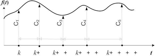
Fig. 3A schematic diagram illustrating the non-uniform embedding process of time series ft into a 5-dimensional delay coordinate space with time delays τ1-τ4 and coordinate axes C1 – C5

A schematic diagram illustrating the non-uniform embedding process of time series ft into a 5-dimensional delay coordinate space with time delays τ1-τ4 and coordinate axes C1 – C5

All possible planar projections of the embedded attractor for time series nv515.dat at $τ_{1} = 1$ ; $τ_{2} = 1$ ; $τ_{3} = 1$ and $τ_{4} = 1$ are depicted in Fig. 3. Analogously, all possible planar projections of the embedded attractor for time series nv515.dat at $τ_{1} = 14$ ; $τ_{2} = 14$ ; $τ_{3} = 33$ and $τ_{4} = 12$ are depicted in Fig. 4.

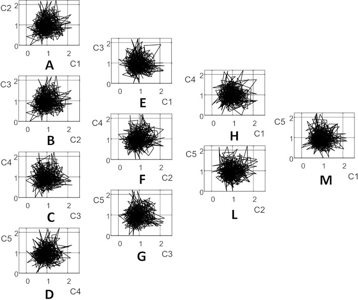
Fig. 4All possible planar projections of the embedded attractor of time series nv515.dat into a 5-dimensional delay coordinate space with time delays τ1=1; τ2=1; τ3=1 and τ4=1. The notations on the axes correspond to the notation used in Fig. 2

All possible planar projections of the embedded attractor of time series nv515.dat into a 5-dimensional delay coordinate space with time delays τ1=1; τ2=1; τ3=1 and τ4=1. The notations on the axes correspond to the notation used in Fig. 2

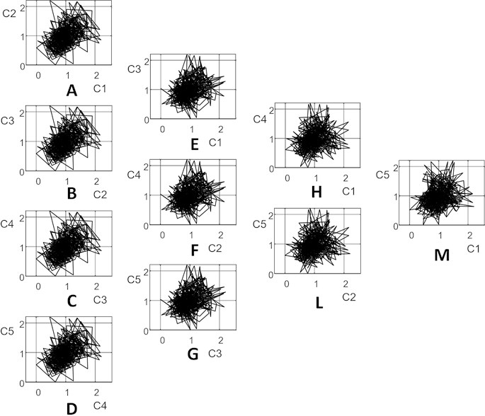
A straightforward comparison between the shapes of the planar projections of the reconstructed attractors in Fig. 3 and Fig. 4 reveals that the projections of the attractor are more compressed along the hypotenuse in Fig. 3 (especially in parts A to D where time delays are equal to 1). The dynamical features of the reconstructed attractor are best revealed when the set of optimal time delays is used for its reconstruction [17] (Fig. 4).

Fig. 5All possible planar projections of the embedded attractor of time series nv515.dat into a 5-dimensional delay coordinate space with optimal time delays τ1=14; τ2=14; τ3=33 and τ4=12. The notations on the axes correspond to the notation used in Fig. 2

All possible planar projections of the embedded attractor of time series nv515.dat into a 5-dimensional delay coordinate space with optimal time delays τ1=14; τ2=14; τ3=33 and τ4=12. The notations on the axes correspond to the notation used in Fig. 2

3.2. Considerations about the optimal embedding dimension

As mentioned previously, the FNN algorithm suggests that the optimal embedding dimension for time series nv515.dat and qbirths.dat is $m = 5$ . However, the embedding dimension should be determined taking into account also the length of the time series [1]. The length of the time series $N$ should be much larger than $m!$ in order for all possible permutations to have a chance to appear [1]. As a rule of thumb, the condition $N > 5 m!$ is widely adopted in the literature as a convention [13].

The lengths of time series nv515.dat and qbirths.dat are 4351 and 5113 correspondingly. Therefore, the condition $N > 5 m!$ is conveniently satisfied for both time series. However, this becomes a serious issue when coarse-grained time series are considered $(i n t (N / s) > 5 m!)$ . Acceptable and unacceptable embeddings for both time series are depicted in Table 1 and Table 2. Note that optimal time delays are determined separately for each embedding dimension $m$ .

It can be observed that acceptable embeddings for time series nv515.dat at $m = 5$ are achieved only if the scale factor $s$ is not larger than 6 (Table 1). Analogously, acceptable embeddings for time series qbirths.dat at $m = 5$ are achieved only if $s < = 8$ . In other words, the discriminant statistic (linear regression coefficient) between MPE and MPWE becomes an unreliable statistical parameter when the scale factor $s$ is varied between 1 and 20 (as defined in [2]).

Table 1Acceptable embeddings for time series nv515.dat. The number of vectors in the trajectory matrix must be higher than 5m! (m is the embedding dimension; s is the scale factor of the coarse-grained time series; N is the length of the original time series). Optimal time delays are: T=44 at m=2; T=44, 50 at m=3; T=46, 45, 50 at m=4; T=14, 14, 33, 12 at m=5; T=28, 23, 22, 46, 23 at m=6. Bold and italic font denote unacceptable embeddings

$s$	$i n t (N / s)$	$m =$ 2	$m =$ 3	$m =$ 4	$m =$ 5	$m =$ 6
1	4351	4307	4257	4210	4278	4209
2	2176	2132	2082	2035	2103	2034
3	1450	1406	1356	1309	1377	1308
4	1088	1044	994	947	1015	946
5	870	826	776	729	797	728
6	725	681	631	584	652	583
7	622	578	528	481	549	480
8	544	500	450	403	471	402
9	483	439	389	342	410	341
10	435	391	341	294	362	293
11	396	352	302	255	323	254
12	363	319	269	222	290	221
13	335	291	241	194	262	193
14	311	267	217	170	238	169
15	290	246	196	149	217	148
16	272	228	178	131	199	130
17	256	212	162	115	183	114
18	242	198	148	101	169	100
19	229	185	135	88	156	87
20	218	174	124	77	145	76
	$5 m!$	10	30	120	600	3600

Table 2Acceptable embeddings for time series qbirths.dat. The number of vectors in the trajectory matrix must be higher than 5m! (m is the embedding dimension; s is the scale factor of the coarse-grained time series; N is the length of the original time series). Optimal time delays are: T=3 at m=2; T=3,1 at m=3; T=1,2,2 at m=4; T=2,1,2,2 at m=5; T=2,2,12,3,30 at m=6. Bold and italic font denote unacceptable embeddings

$s$	$i n t (N / s)$	$m =$ 2	$m =$ 3	$m =$ 4	$m =$ 5	$m =$ 6
1	5113	5110	5109	5108	5106	5064
2	2557	2554	2553	2552	2550	2508
3	1704	1701	1700	1699	1697	1655
4	1278	1275	1274	1273	1271	1229
5	1023	1020	1019	1018	1016	974
6	852	849	848	847	845	803
7	730	727	726	725	723	681
8	639	636	635	634	632	590
9	568	565	564	563	561	519
10	511	508	507	506	504	462
11	465	462	461	460	458	416
12	426	423	422	421	419	377
13	393	390	389	388	386	344
14	365	362	361	360	358	316
15	341	338	337	336	334	292
16	320	317	316	315	313	217
17	301	298	297	296	294	252
18	284	281	280	279	277	235
19	269	266	265	264	262	220
20	256	253	252	251	249	207
	5 $m!$	10	30	120	600	3600

Without doubts, the optimal embedding dimension $m = 5$ should be used for both time series (nv515.dat and qbirths.dat) if only the data records would be long enough. The length of the time series must be taken into account when making a decision about the acceptable embedding dimension [1]. Table 1 and Table 2 suggest that $m = 4$ would be a good compromise for both time series.

4. The comparison between the discriminant statistic and the modified discriminant statistic

The algorithm presented in [2] is executed for both time series (nv515.dat and qbirths.dat) at $m = 5$ and $T = \{1,1, 1,1\}$ . Relationships between MPE and MPWE are depicted in Fig. 5. The discriminant statistic (linear regression coefficient) between MPE and MPWE for time series nv515.dat at $T = \{1,1, 1,1\}$ is 0.6665 (Fig. 5(a)); linear regression coefficient between MPE and MPWE for time series qbirths.dat at $T = \{1, 1, 1, 1\}$ is 0.6639 (Fig. 5(b)). As noted previously, such computations are unreliable because the condition $i n t (N / s) > 5 m!$ does not hold true for all s (gray circles denote such MPE – MPWE points where the condition is broken).

Fig. 6The discriminant statistic presented in [2] cannot determine a large difference between time series nv515.dat and qbirths.dat at m=5. The modified discriminant statistic (based on optimal embedding parameters) shows a large difference between time series nv515.dat and qbirths.dat at m=4. Linear regressions between MPE and MPWE for nv515.dat and qbirths.dat at T=1,1,1,1, m=5 are shown in parts A and B respectively. Linear regressions between MPE and MPWE for nv515.dat (at T=46,45,50) and for qbirths.dat (at T=1,2,2) at m=4 are shown in parts C and D respectively. Gray circles denote unreliable embeddings when the condition int(N/s)>5m! does not hold true

The discriminant statistic presented in [2] cannot determine a large difference between time series nv515.dat and qbirths.dat at m=5. The modified discriminant statistic (based on optimal embedding parameters) shows a large difference between time series nv515.dat and qbirths.dat at m=4. Linear regressions between MPE and MPWE for nv515.dat and qbirths.dat at T=1,1,1,1, m=5 are shown in parts A and B respectively. Linear regressions between MPE and MPWE for nv515.dat (at T=46,45,50) and for qbirths.dat (at T=1,2,2) at m=4 are shown in parts C and D respectively. Gray circles denote unreliable embeddings when the condition int(N/s)>5m! does not hold true

Computational experiments are continued at $m = 4$ and optimal time delays $T = \{46,45,50\}$ (nv515.dat) and $T = \{1, 2, 2\}$ (qbirths.dat). The discriminant statistic (linear regression coefficient) between MPE and MPWE for time series nv515.dat is 0.5539 (Fig. 5(c)); linear regression coefficient between MPE and MPWE for time series qbirths.dat is 0.4728 (Fig. 5(d)).

5. Computational simulations with synthetic data

Computational simulations are continued with the chaotic Rössler system which is a paradigmatic model of chaotic dynamics [12]:

9

\{\begin{array}{l} \frac{d x}{d t} = - y - z, \\ \frac{d y}{d t} = x + a y, \\ \frac{d z}{d t} = b + z (x - c), \end{array}

where constants $a$ , $b$ , $c$ are set to $a =$ 0.1, $b$ = 0.1, $c$ = 14. The Rössler time series is generated by integrating the system of equations in Eq. (9) and by selecting every tenth value of $x$ (the time step is set to 0.01). Different realizations of the discrete Gaussian random noise with zero mean are added to the synthetic Rössler time series. Optimal embedding dimensions and optimal time lags for the Rössler time series with 10 %, 50 % and 200 % noise levels are shown in Table 3 [16].

Table 3Optimal embedding dimensions, optimal time lags [16], the discriminant statistic, the mean of the modified discriminant statistic for the Rössler time series with different noise levels

Noise level	Optimal embedding dimension	Optimal time lags	The discriminant statistic $β$	The mean of the modified discriminant statistic $\hat{β}$	The confidence interval
10 %	6	{37, 45, 17, 38, 6}	0.9474	0.8754	[0.8521; 0.8987]
50 %	7	{36, 16, 14, 28, 35, 36}	0.9840	0.9987	[0.991; 1.0064]
200 %	8	{49, 41, 15, 36, 33, 16, 40}	0.9943	1.0238	[1.0195; 1.0281]

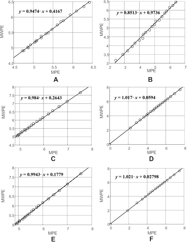
Linear regressions between MPE and MPWE for the Rössler time series with 10 %, 50 % and 200 % noise levels (all time lags are set to 1) are shown in Fig. 6(a, c, e). Linear regressions at non-uniform embeddings with optimal time lags are shown in Fig. 6(b, d, f). The discriminant statistic $β$ (reconstructed by using uniform embedding) and the modified discriminant statistic $\hat{β}$ (reconstructed by using non-uniform embedding) are shown in Table 3.

Two important conclusions can be done from the results depicted in Table 6. Firstly, the modified discriminant statistic $\hat{β}$ is able to determine larger differences between different time series. Secondly, the difference between $β$ and $\hat{β}$ becomes smaller as the noise level becomes larger. This fact does correspond well to the fact that any time delays are equally good (in terms of the area occupied by the embedded attractor in the delay coordinate space) if the embedded time series is the white noise [17].

It is also important to evaluate the uncertainty of the modified discriminant statistic $\hat{β}$ . As discussed previously, the real-world time series nv515.dat and qbirths.dat are relatively short (Fig. 5). However, the chaotic Rössler time series is generated using computational algorithms without any restrictions in its length. Therefore, the slope coefficients (the modified discriminant statistic $\hat{β}$ ) is computed ten consecutive times in ten non-overlapping observation windows. The confidence interval for $\hat{β}$ using the three-sigma rule ( $p$ = 0.05) is computed according to the results of repetitive computational experiments.

The confidence intervals of $\hat{β}$ for the Rössler time series with 10 % noise, 50 % noise, and 200 % noise are [0.8521; 0.8987], [0.991; 1.0064], [1.0195; 1.0281] accordingly. It is interesting to observe that the discriminant statistic $β$ stays outside the confidence intervals of $\hat{β}$ (Table 3). This is a rather natural and expected results because the chaotic Rössler time series is a stationary ergodic time series [11]. Of course, the situation would be different if the analyzed time series would be non-stationary time series (the value of $\hat{β}$ would depend on the location of the observation window).

Fig. 7Linear regressions between MPE and MPWE for the Rössler time series with 10 %, 50 % and 200 % noise levels (all time lags are set to 1) are shown in Fig. 6 parts A, C, and E. Linear regressions for the Rössler time series with 10 %, 50 % and 200 % noise levels (optimal non-uniform time lags are set according to Table 1) are shown in Fig. 6 parts B, D, and F

Linear regressions between MPE and MPWE for the Rössler time series with 10 %, 50 % and 200 % noise levels (all time lags are set to 1) are shown in Fig. 6 parts A, C, and E. Linear regressions for the Rössler time series with 10 %, 50 % and 200 % noise levels (optimal non-uniform time lags are set according to Table 1) are shown in Fig. 6 parts B, D, and F

6. Discussions

The main objective of this paper is to demonstrate that the selection of optimal time delay(s) is an essential step in the application of discriminant statistic based on the relation between MPE and MWPE.

The objective of time delay selection methods is making components of the reconstructed vectors independent as far as possible – yet not too far, in order to keep the information about dynamic properties of the embedded time series. Moreover, optimal time lags do also result into the maximal area (in average) in all possible planar projections of the embedded attractor. Setting all time delays to 1 results into higher correlations between the components of the reconstructed vectors – what has a direct impact to the computation of MPE and MWPE. Convincing demonstrations of these effects are given in Figs. 3 and 4.

The optimization of time delays can be ignored if the time series is random, or the signal to noise ratio is very low. As mentioned previously, the selection of particular time delays is meaningless if the embedded time series does represent a random noise. Otherwise, the geometric shape of embedded attractors (and the patterns of components of the reconstructed vectors) do depend on time delays.

For example, the shapes of the planar attractors in Fig. 3 are more compressed along the diagonal if compared to Fig. 4 (this effect is especially clearly seen in parts A to D). In other words, the components of the reconstructed vectors in the trajectory matrix are more correlated in Fig. 3 than in Fig. 4.

This effect is clearly represented in the discriminant statistic based on the relation between MPE and MWPE (Fig. 5). The discriminant statistic does not show a big difference between time series nv515.dat and qbirths.dat when all time delays are set to 1. The percentage difference between the two discriminant statistic values is 0.39 % (0.6665 versus 0.6639). However, the discriminant statistic shows a much higher percentage difference when time delays are optimal: 14.64 % (0.5539 versus 0.4728).

Spearman's rank correlation coefficient is used to assess how well the relationship between MPE and MPWE can be described using a linear function. Note that a linear fit between the two variables is better for time series nv515.dat than qbirths.dat (Fig. 5). Short optimal time delays for time series qbirths.dat $\{1, 2, 2\}$ show that independent components of the trajectory matrix cannot be separated far away without destroying the information about dynamic properties of the embedded time series. Of course, a thorough investigation of the search space of time delays would be required to identify how strong is the global maximum $\{1, 2, 2\}$ in respect to other local maximums. That would help to determine how different is this time series from the random noise [17]. Nevertheless, the fact that Spearman’s rank correlation coefficient for births.dat is lower than for nv515.dat is not astonishing. On the other hand, the comparison of Spearman’s rank correlation coefficient for Fig. 5(b) and Fig. 5(d) is meaningless because computational experiments depicted in Fig. 5(b) are based on unacceptable embeddings.

Fig. 8Two-dimensional patterns of PE for nv515.dat time series (m= 5; T= 14, 14, 33, 12). Pairwise relaxation of time delays [A] results into six plane images: 14,14,i,j (part A); 14,i,33,j (part B); 14,i,j,12 (part C); i,14,33,j (part D); i,14,j,12 (part E); i,j,33,12 (part F) ); i,j= 1...50. The average of all six parts is shown in part G

Two-dimensional patterns of PE for nv515.dat time series (m= 5; T= 14, 14, 33, 12). Pairwise relaxation of time delays [A] results into six plane images: 14,14,i,j (part A); 14,i,33,j (part B); 14,i,j,12 (part C); i,14,33,j (part D); i,14,j,12 (part E); i,j,33,12 (part F) ); i,j= 1...50. The average of all six parts is shown in part G

Optimal non-uniform time delays can be also useful for estimating basic ordinal quantifiers (PE, WPE, MPE, WMPE) – not only the proposed discriminant statistic based on the relation between MPE and WMPE. However, optimal non-uniform time delays are also useful for the extraction of much more complex ordinal features (two-dimensional patterns of PE could be a typical application discussed in detail in [16, 7].

In other words, feature extraction algorithms based on ordinal quantifiers can be conditionally classified into the following multiscale structure according to their complexity. The basic ordinal quantifiers (PE, WPE, MPE, WMPE) could be considered as the basic elements of such a multiscale feature extraction structure. The discriminant statistic (relating MPE and MWPE) can be placed in the middle of this multiscale structure. Finally, two-dimensional patterns of PE would be the most complex elements in this structure of ordinal quantifiers.

Fig. 9Two-dimensional patterns of PE for qbirths.dat time series (m= 5; T= 2, 1, 2, 2). Pairwise relaxation of time delays [A] results into six plane images: 2,1,i,j (part A); 2,i,2,j (part B); 2,i,j,2 (part C); i,1,2,j (part D); i,1,j,2 (part E); i,j,2,2 (part F) ); i,j= 1...50. The average of all six parts is shown in part G

Two-dimensional patterns of PE for qbirths.dat time series (m= 5; T= 2, 1, 2, 2). Pairwise relaxation of time delays [A] results into six plane images: 2,1,i,j (part A); 2,i,2,j (part B); 2,i,j,2 (part C); i,1,2,j (part D); i,1,j,2 (part E); i,j,2,2 (part F) ); i,j= 1...50. The average of all six parts is shown in part G

Two-dimensional patterns of PE for nv515.dat and qbirths.dat time series are depicted in Fig. 7(g) and Fig. 8(g) accordingly (the resolution of those patterns is set to 50×50 pixels). As mentioned previously, the optimal embedding dimension for both time series is $m =$ 5 (the set of optimal time delays for nv515.dat is $T =$ 14, 14, 33, 12; the set of optimal time delays for qbirths.dat is $T =$ 2, 1, 2, 2). Pairwise relaxation of time delays [16] results into six plane images for each time series: 14,14,i,j (Fig. 7(a)); 14,i,33,j (Fig. 7(b)); 14,i,j,12 (Fig. 7(c)); i,14,33,j (Fig. 7(d)); i,14,j,12 (Fig. 7(e)); i,j,33,12 (Fig. 7(f)); 2,1,i,j (Fig. 8(a)); 2,i,2,j (Fig. 8(b)); 2,i,j,2 (Fig. 8(c)); i,1,2,j (Fig. 8(d)); i,1,j,2 (Fig. 8(e)); i,j,2,2 (Fig. 8(f)); $i$ , $j =$ 1,...,50. It is shown in [7] that deep learning based convolutional neural networks can classify the averaged patterns of PE (Fig. 7(g) and Fig. 8(g)) with an extremely high accuracy. Indeed, a naked eye can observe clear differences between Fig. 7(g) and Fig. 8(g).

The main objective of this article is to highlight the fact that non-uniform time delays play a central role not only at the top level (in terms of complexity) of ordinal quantifiers. A proper assessment of optimal time delays is crucial also in the middle level of this structure (the discriminant statistic). The latter observation is even more important because the original discriminant statistic presented in [2] does not pay any attention to non-uniform embeddings.

7. Conclusions

Some problems regarding the use of non-overlapping windows for coarse graining, for the original MSE algorithm, are addressed in [4]. For example, the embedding problems related to the length of the time series could be almost completely eliminated if the coarse-grained time series would be constructed using overlapping windows. However, such a construction of a coarse-grained time series would result into a simple moving average – what would induce another problems discussed in [8]. Therefore, the construction of coarse-grained time series in this paper is performed using non-overlapping windows only.

The discriminant statistic presented in [2] is an interesting statistical parameter which can be used to characterize time series. However, this discriminant statistic is a result of a statistical algorithm. Therefore, it must be used with care (that statement holds true for any statistical algorithm in general). In particular, one should determine the optimal embedding dimension and the optimal set of time delays before running this algorithm for any time series.

In any case, it is always recommended to couple feature extraction algorithms based on ordinal quantifiers with the optimal parameters of non-uniform embeddings (the optimal embedding dimension and the optimal set of non-uniform time delays).

References

C. Bandt and B. Pompe, “Permutation entropy: a natural complexity measure for time series,” Physical Review Letters, Vol. 88, No. 17, p. 174102, Apr. 2002, https://doi.org/10.1103/physrevlett.88.174102

Publisher
S. Chen and P. Shang, “Financial time series analysis using the relation between MPE and MWPE,” Physica A: Statistical Mechanics and its Applications, Vol. 537, p. 122716, Jan. 2020, https://doi.org/10.1016/j.physa.2019.122716

Publisher
B. Fadlallah, B. Chen, A. Keil, and J. Príncipe, “Weighted-permutation entropy: A complexity measure for time series incorporating amplitude information,” Physical Review E, Vol. 87, No. 2, p. 022911, Feb. 2013, https://doi.org/10.1103/physreve.87.022911

Publisher
A. Humeau-Heurtier, “The multiscale entropy algorithm and its variants: a review,” Entropy, Vol. 17, No. 5, pp. 3110–3123, May 2015, https://doi.org/10.3390/e17053110

Publisher
R. Hyndman and Y. Yang. “Time series data library.” pkg.yangzhuoranyang.com/tsdl.

Search CrossRef
M. B. Kennel, R. Brown, and H. D. I. Abarbanel, “Determining embedding dimension for phase-space reconstruction using a geometrical construction,” Physical Review A, Vol. 45, No. 6, pp. 3403–3411, Mar. 1992, https://doi.org/10.1103/physreva.45.3403

Publisher
M. Landauskas, M. Cao, and M. Ragulskis, “Permutation entropy-based 2D feature extraction for bearing fault diagnosis,” Nonlinear Dynamics, Vol. 102, No. 3, pp. 1717–1731, Nov. 2020, https://doi.org/10.1007/s11071-020-06014-6

Publisher
M. Landauskas, Z. Navickas, A. Vainoras, and M. Ragulskis, “Weighted moving averaging revisited: an algebraic approach,” Computational and Applied Mathematics, Vol. 36, No. 4, pp. 1545–1558, Dec. 2017, https://doi.org/10.1007/s40314-016-0309-9

Publisher
K. Lukoseviciute and M. Ragulskis, “Evolutionary algorithms for the selection of time lags for time series forecasting by fuzzy inference systems,” Neurocomputing, Vol. 73, No. 10-12, pp. 2077–2088, Jun. 2010, https://doi.org/10.1016/j.neucom.2010.02.014

Publisher
Y. Manabe and B. Chakraborty, “A novel approach for estimation of optimal embedding parameters of nonlinear time series by structural learning of neural network,” Neurocomputing, Vol. 70, No. 7-9, pp. 1360–1371, Mar. 2007, https://doi.org/10.1016/j.neucom.2006.06.005

Publisher
M. Ragulskis and K. Lukoseviciute, “Non-uniform attractor embedding for time series forecasting by fuzzy inference systems,” Neurocomputing, Vol. 72, No. 10-12, pp. 2618–2626, Jun. 2009, https://doi.org/10.1016/j.neucom.2008.10.010

Publisher
O. E. Rössler, “An equation for continuous chaos,” Physics Letters A, Vol. 57, No. 5, pp. 397–398, Jul. 1976, https://doi.org/10.1016/0375-9601(76)90101-8

Publisher
M. Riedl, A. Müller, and N. Wessel, “Practical considerations of permutation entropy,” The European Physical Journal Special Topics, Vol. 222, No. 2, pp. 249–262, Jun. 2013, https://doi.org/10.1140/epjst/e2013-01862-7

Publisher
T. Sauer, J. A. Yorke, and M. Casdagli, “Embedology,” Journal of Statistical Physics, Vol. 65, No. 3-4, pp. 579–616, Nov. 1991, https://doi.org/10.1007/bf01053745

Publisher
T. Schreiber, “Interdisciplinary application of nonlinear time series methods,” Physics Reports, Vol. 308, No. 1, pp. 1–64, Jan. 1999, https://doi.org/10.1016/s0370-1573(98)00035-0

Publisher
M. Tao, K. Poskuviene, N. Alkayem, M. Cao, and M. Ragulskis, “Permutation entropy based on non-uniform embedding,” Entropy, Vol. 20, No. 8, p. 612, Aug. 2018, https://doi.org/10.3390/e20080612

Publisher
I. Timofejeva, K. Poskuviene, M. Cao, and M. Ragulskis, “Synchronization measure based on a geometric approach to attractor embedding using finite observation windows,” Complexity, Vol. 2018, pp. 1–16, Aug. 2018, https://doi.org/10.1155/2018/8259496

Publisher
Y. Yin and P. Shang, “Weighted multiscale permutation entropy of financial time series,” Nonlinear Dynamics, Vol. 78, No. 4, pp. 2921–2939, Dec. 2014, https://doi.org/10.1007/s11071-014-1636-2

Publisher
M. Zanin, L. Zunino, O. A. Rosso, and D. Papo, “Permutation entropy and its main biomedical and econophysics applications: a review,” Entropy, Vol. 14, No. 8, pp. 1553–1577, Aug. 2012, https://doi.org/10.3390/e14081553

Publisher

Cited by

Multiscale Cumulative Residual Dispersion Entropy with Applications to Cardiovascular Signals

Youngjun Kim | Young-Seok Choi

(2023)

About this article

Received

08 June 2022

Accepted

30 August 2022

Published

27 September 2022

DOI

https://doi.org/10.21595/jme.2022.22897

Keywords

time series

permutation entropy

attractor embedding

Acknowledgements

The authors are grateful for the International Science & Technology Cooperation Project of Jiangsu Province (BZ2022010), the Nanjing International Joint Research and Development Program (No. 202112003), and the Nantong Science and Technology Opening Cooperation Project (No. BW2021001).

Data Availability

The datasets generated during and/or analyzed during the current study are available from the corresponding author on reasonable request.

Conflict of interest

The authors declare that they have no conflict of interest.

This is an open access article distributed under the Creative Commons Attribution License, which permits unrestricted use, distribution, and reproduction in any medium, provided the original work is properly cited.

Previous article in issue Previous

Research article

2021 08 11

Gear compound fault detection method based on improved multiscale permutation entropy and local mean decomposition

Yongqi Chen, Yang Chen, Qinge Dai

Research article

2019 11 15

Fault diagnosis using an improved fusion feature based on manifold learning for wind turbine transmission system

Ping Ma, Hongli Zhang, Wenhui Fan, Cong Wang

Research article

2019 10 19

Fault identification technology for gear tooth surface wear based on MPE method by MI and improved FNN algorithm

Xintao Zhou, Yahui Cui, Xiayi Liu, Longlong Li, Lihua Wang

Research article

2018 03 31

Novel bearing fault diagnosis model integrated with dual-tree complex wavelet transform, permutation entropy and optimized FCM

Ping Ma, Hongli Zhang, Wenhui Fan, Cong Wang

V. Petrauskiene, J. Ragulskiene, H. Zhu, J. Wang, and M. Cao, “The discriminant statistic based on MPE-MWPE relationship and non-uniform embedding,” Journal of Measurements in Engineering, Vol. 10, No. 3, pp. 150–163, Sep. 2022, https://doi.org/10.21595/jme.2022.22897

Copy Extrica

Copied to clipboard!

TY  - JOUR
DO  - 10.21595/jme.2022.22897
UR  - https://doi.org/10.21595/jme.2022.22897
TI  - The discriminant statistic based on MPE-MWPE relationship and non-uniform embedding
T2  - Journal of Measurements in Engineering
AU  - Petrauskiene, Vilma
AU  - Ragulskiene, Jurate
AU  - Zhu, Huaxin
AU  - Wang, Jie
AU  - Cao, Maosen
PY  - 2022
DA  - 2022/09/27
PB  - JVE International Ltd.
SP  - 150-163
VL  - 10
IS  - 3
SN  - 2335-2124
SN  - 2424-4635
ER  - 

Copy Ris

Copied to clipboard!

@article{Petrauskiene_2022,
	doi = {10.21595/jme.2022.22897},
	url = {https://doi.org/10.21595/jme.2022.22897},
	year = 2022,
	month = {sep},
	publisher = {{JVE} International Ltd.},
	volume = {10},
	number = {3},
	pages = {150--163},
	author = {Vilma Petrauskiene and Jurate Ragulskiene and Huaxin Zhu and Jie Wang and Maosen Cao},
	title = {The discriminant statistic based on {MPE}-{MWPE} relationship and non-uniform embedding},
	journal = {Journal of Measurements in Engineering}
}

Copy Bibtex

Copied to clipboard!

[1]V. Petrauskiene, J. Ragulskiene, H. Zhu, J. Wang, and M. Cao, “The discriminant statistic based on MPE-MWPE relationship and non-uniform embedding,” Journal of Measurements in Engineering, vol. 10, no. 3, pp. 150–163, Sep. 2022, doi: 10.21595/jme.2022.22897.

Copy IEEE

Copied to clipboard!

Petrauskiene, Vilma, Jurate Ragulskiene, Huaxin Zhu, Jie Wang, and Maosen Cao. “The Discriminant Statistic Based on MPE-MWPE Relationship and Non-Uniform Embedding.” Journal of Measurements in Engineering 10, no. 3 (September 27, 2022): 150–63. https://doi.org/10.21595/jme.2022.22897.

Copy Chicago

Copied to clipboard!

The discriminant statistic based on MPE-MWPE relationship and non-uniform embedding

Abstract

1. Introduction

2. Preliminaries

2.1. Permutation entropy and weighted permutation entropy

2.2. Multi-scale permutation entropy

2.3. Linear regression between MPE and WMPE

3. The selection of optimal embedding parameters

3.1. Optimal non-uniform embeddings of two real-world time series

3.2. Considerations about the optimal embedding dimension

4. The comparison between the discriminant statistic and the modified discriminant statistic

5. Computational simulations with synthetic data

6. Discussions

7. Conclusions

References

Cited by

About this article

Related Articles