Numerical simulation of the supercritical carbon dioxide flow in converted marine pipelines

1. Introduction

Reducing the level of carbon dioxide emissions into the atmosphere is one of the priorities of the energy sector of developed countries. One of the ways to solve this issue is the direct capture of harmful substances from factories and industrial facilities. There are three types of capture, depending on the stage at which the collection takes place: pre-combustion, post-combustion and oxy-fuel. The degree of purity of the captured carbon dioxide and the component composition of the resulting gas depend on the chosen method [1].

The most common method of utilization of captured carbon dioxide is its injection into depleted deposits and salt caverns [2, 3]. The choice of the most suitable phase state for injection is determined by the conditions of a particular production facility and the existing infrastructure. The preferred conditions are pumping in the supercritical phase with pre-drying in order to minimize the risks of corrosion on the metal of the pipe. In this case, an important task is to determine the critical parameters of the fluid, which strongly depend on the components included in the composition [4]. An example of a phase envelope for post-combustion capture is shown in Fig. 1. Vapour-Liquid Equilibrium and Water lines are depicted as wells as Critical Point (C) and Dew Point (D).

Fig. 1A phase envelope for the post-combustion flow

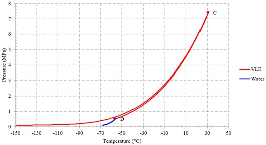
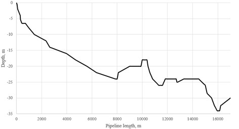
To ensure pumping in a supercritical state, the fluid pressure and temperature must always be in the zone to the right of point C. Within the framework of this work, pumping through the existing offshore pipeline connecting the offshore platform and the coastal complex is considered. Thus, the conversion of the original pipeline is ensured. The geometry of the pipeline is presented at Fig. 2. The pipeline has internal diameter of 327 mm and the wall thickness of 14,5 mm and two extra layers: 6 mm of bitumen enamel to isolate the steel and 71 mm of concrete to fix the position. It is laid at the bottom of the trench with the average 1 m of burial. The 1:0 slope and cofferdam wall construction method are used. The total length is 17,5 km. The flow rate in the pipe is determined by the level of carbon dioxide captured from hydrogen production plants located near the platform.

Fig. 2The studied marine pipeline geometry

2. Calculation model

The question of the correctness of the calculation of pressure losses in multiphase and supercritical pipelines laid over rough terrain was considered by many authors [5, 6]. Summing up the information, it can be concluded that the pressure drop is calculated by the following formula:

where ${∆P}_{fr}$ – friction pressure drop, ${∆P}_{ac}$ – acceleration pressure drop and ${∆P}_g$ – pressure drop due to the gravity.

The named components are calculated by the following formulas:

where $G$ – mass flux, kg/(m²∙s); $\rho$ – fluid density, kg/m³; $L$ – tube length, m; $D$ – inner diameter, m; $f$ – friction factor; $f_{ac}$ – acceleration factor; $\theta$ – pipe inclination angle.

The sign “+” is for the upward flow, and the sign “–” is for the downward flow.

The supercritical friction factor f is not to be confused with the friction coefficient, sometimes called the Fanning friction factor:

where $f_{iso,b}$ – isothermal single-phase friction factor at fluid bulk temperature; ${\mu }_w$, ${\mu }_b$ – dynamic viscosity at inner wall temperature and fluid bulk temperature respectively, Pa∙s; ${\rho }_f$, ${\rho }_{pc}$ – fluid density at film temperature and pseudo-critical temperature respectively, kg/m³.

For cooling processes, $f_{ac}$ can be approximated with the one-dimensional approximation mode:

where ${\rho }_b$ – fluid density at fluid bulk temperature, kg/m³; $q$ – heat flux from fluid to wall, W/m²; $\beta$ – thermal expansion coefficient at fluid bulk temperature, 1/K; $C_p$ – specific heat at constant pressure, J/(kg∙K).

The calculated dependences and equations created for modeling the fluid flow process in the pipeline can be divided depending on the method of their development. Empirical and mechanistic models are distinguished. According to the general principles of modeling, the first models contain many dimensionless complexes, but this imposes certain restrictions on their applicability to real problems (Beggs&Brill, Orkiszewski). On the other hand, mechanistic ones are related to the direct solution of the equation of fluid motion (Tulsa Unified Model, OLGAS, HTFS). Despite their high accuracy, the simulation results may still be unstable when simulating conditions beyond the initial working area. In this study, the mechanistic approach is applied.

Fig. 3Pressure distribution along the pipeline at τ= 0 (model 1)

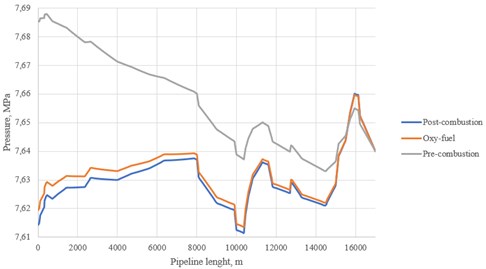
Fig. 4Pressure distribution along the pipeline at τ= 0 (model 2)

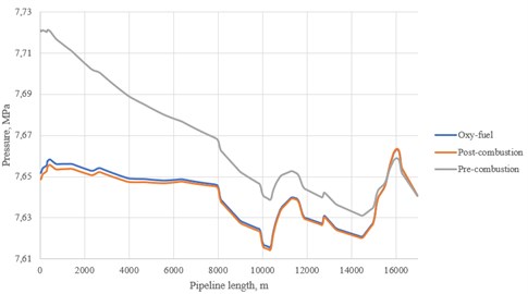
Steady state calculation of pressure and temperature distribution was made using mechanistic approach. The case was to find the proper pressure and temperature at inlet if the same parameters at the outlet were known and provide SCF state. The pressure at the outlet was set at 7,64 MPa to cover the maximum critical value, the temperature was set at 32 °C (Fig. 3-6). The outlet temperature for pre-combustion stream was set at 33 °C due to convergence limitations. Two different correlations were applied to compare the results.

Fig. 5Temperature distribution along the pipeline at τ= 0 (model 1)

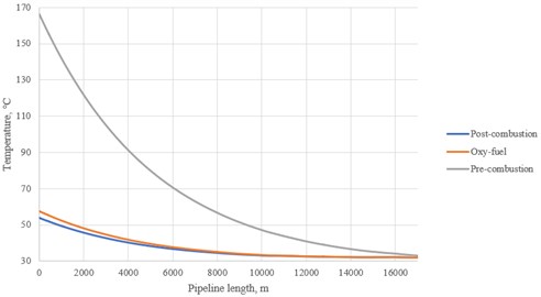
Fig. 6Temperature distribution along the pipeline at τ= 0 (model 2)

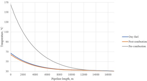
The resulting graphs at initial moment of time ($\tau =$0) clearly show a significant difference in the behavior of streams of different origin. Pressure and temperature levels for the pre-combustion flow are much higher than the ones for oxy-fuel and post-combustion due to the relatively high degree of contamination (Table 1). Despite the named aspect, all the cases can be implemented due to the fact that the maximum operating pressure (MOP) and maximum allowable operating pressure (MAOP) levels were not exceeded. Reference values are 9,1/9,8 MPa and 10 MPa respectively. However, the obtained values of temperature for pre-combustion stream are much higher than mean operating temperature of oil or gas. Reference values are 12,5 °C and 5 °C respectively. The results of modelling are presented at Table 1.

Analyzing the results, it can be established that the second calculation model shows larger values. However, the inlet temperature for pre-combustion is slightly lower for this correlation.

The resulting SCF flows are not stable if the change of parameters in time is considered. To track changes in the state of the system over time, the second model was applied due to its high efficiency for dynamic tasks. The problem was solved for a period of 72 hours. Results of modelling at certain points of time are presented at Figs. 7-12.

Fig. 7Pressure distribution for the pre-combustion flow

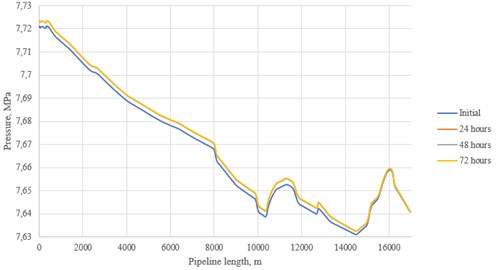
Fig. 8Pressure distribution for the post-combustion flow

Fig. 9Pressure distribution for the oxy-fuel flow

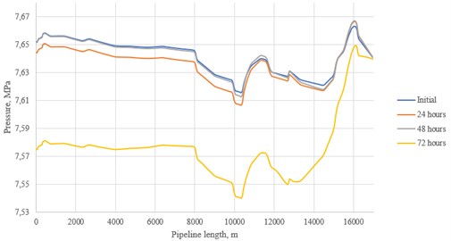
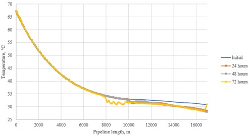
According to the received schedules of changes, the following conclusions can be drawn. The oxy-fuel flow is subject to the greatest fluctuations: this is especially noticeable at 72 hours after the start of the simulation, when the pressure in the pipeline drops significantly along its entire length, and the temperature curve acquires a wave character at the point of local elevation of the route. In the latter case, there is a drop in the operating temperature below the critical value, which leads to the appearance of a liquid phase. As for the post-combustion flow, fluctuations in pressure also occurred, especially in the shallowest part of the pipeline route. The pre-combustion one turned out to be the most stable flow due to the comparatively high temperature values. One of the possible ways to stabilize the flow is to increase the pumping speed to the recommended value of 2 m/s [7]. This can be achieved by increasing the mass flow of air in the case of CO₂ capture from nearby industrial facilities.

Fig. 10Temperature distribution for the pre-combustion flow

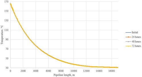
Fig. 11Temperature distribution for the post-combustion flow

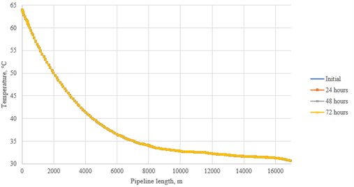
Fig. 12Temperature distribution for the post-combustion flow

Taking into account all the data obtained, the following points should be noted. Among three considered streams of different origin, the most optimal for use is post-combustion. Pre-combustion stream requires extremely high temperatures, and the existing pipelines are initially not designed for such thermal loads. Oxy-fuel option is the least stable one, which can lead to a change in the flow pattern in the pipeline with the slightest change in operating parameters.

3. Conclusions

The calculation of the necessary parameters for pumping supercritical carbon dioxide remains a difficult task due to the lack of a significant experimental base with which the obtained simulation results should be correlated. At the moment, many studies are being conducted, the purpose of which is to determine the most accurate numerical correlation for the flow of a supercritical fluid for any geometry feature. Taking into account the fact that more and more natural reservoirs will become depleted in the next 20-30 years, the issue of reconfiguring the existing infrastructure for back injection into the reservoir is extremely relevant. The issue of a comprehensive study of pipelines remains open, thereof attention should be paid to the influence of converted fluid on residual deposits, pumping equipment and other aspects of operation. If a universal conversion standard is developed, effective disposal will be possible yielding in achieved zero emission goals.

References

-
T. Hickem and S. Siew, Carbon Capture Utilisation and Storage. Singapore: 350 Singapore, 2019.
P. Kosowski and M. Kuk, “Cost analysis of geological sequestration of CO2,” AGH Drilling, Oil, Gas, Vol. 33, No. 1, p. 105, 2016, https://doi.org/10.7494/drill.2016.33.1.105
A. Bielinski, A. Kopp, H. Schutt, and H. Class, “Monitoring of CO2 plumes during storage in geological formations using temperature signals: Numerical investigation,” International Journal of Greenhouse Gas Control, Vol. 2, No. 3, pp. 319–328, Jul. 2008, https://doi.org/10.1016/j.ijggc.2008.02.008
H. Li and J. Yan, “Impacts of equations of state (EOS) and impurities on the volume calculation of CO2 mixtures in the applications of CO2 capture and storage (CCS) processes,” Applied Energy, Vol. 86, No. 12, pp. 2760–2770, Dec. 2009, https://doi.org/10.1016/j.apenergy.2009.04.013
X. Fang, Y. Xu, X. Su, and R. Shi, “Pressure drop and friction factor correlations of supercritical flow,” Nuclear Engineering and Design, Vol. 242, No. 1, pp. 323–330, Jan. 2012, https://doi.org/10.1016/j.nucengdes.2011.10.041
S. Peletiri, N. Rahmanian, and I. Mujtaba, “CO2 Pipeline Design: A Review,” Energies, Vol. 11, No. 9, p. 2184, Aug. 2018, https://doi.org/10.3390/en11092184
About this article
The authors have not disclosed any funding.
The datasets generated during and/or analyzed during the current study are available from the corresponding author on reasonable request.
The authors declare that they have no conflict of interest.