Kinematic analysis and trajectory planning for a tree planting robot in forest environment

1. Introduction

Domestic forestry operations today still rely on human labor to get the job done, especially drilling deep afforestation, which is done by hand. This method is not only time-consuming, but also labor-intensive and inefficient, greatly reducing the speed of afforestation [1-3]. Forest tree planting is a complex undertaking, with labor costs generally account for more than 60 % to 80 % of the actual cost. Labor force is also facing a phase of transformation from manual labor to skilled labor, with the cost of manual labor increasing year on year [4-6]. Considering the increase in labor costs, available labor is limited, and production costs are increasing, therefore, TPRs are urgently needed to perform and simplify these field construction operations mechanically. In addition, as people’s living standards improve and their demand for timber increases, the rate of artificial afforestation is not yet as fast as the growth of people's demand for timber [7]. There has been some research and applications in addressing the inverse kinematics and path planning of robots. However, these studies have focused on industrial robots in unconstrained workspaces with homogeneous objects. TPRs integrate sensing tests, simulation calculations, manipulation and control systems to perform forest tree planting operations with artificial intelligence technology. Moreover, the successful adoption of these technologies requires a combination of the TPR's capabilities and the environment in which it operates in the forest. The environment in which trees are planted is known to be complex. TPR and end effectors attributed to them are likely to collide with adjacent branch obstacles, thus reducing the efficiency of tree planting. The application of TPR technology in forestry operating environments faces considerable challenges. In order to successfully adopt robots in forestry, it is necessary to develop an efficient motion planning algorithm that allows TPRs to complete tree planting tasks.

Forestry is a constrained and dynamic environment with working objects of varying shapes, sizes, positions and orientations. The target attitude of the TPR in each planting task is unknown and the path from the starting point to the target point needs to be re-planned for each target point of the planting task. Furthermore, in order to meet the picking efficiency of TPR, the computational speed of the motion planning algorithm should be motion planning algorithm should be high. Therefore, in order to meet the above requirements, not only a motion planning algorithm is required, but also a motion planning algorithm. The motion planning algorithm for TPR needs to solve not only the inverse kinematic problem of obtaining picking poses for tree picking through a small number of iterations, but also to obtain picking poses through a small number of iterations based on information about the forest environment, and to determine the picking path quickly enough to avoid collisions between the TPR and branching obstacles.

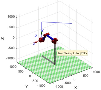
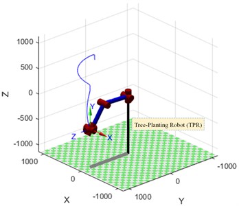
This study is based on the above considerations, a motion path planning method for TPR based on the above research is proposed, the simulation results confirm that the proposed motion planning method enables the TPR to avoid obstacles in the workspace and to complete the tree planting task efficiently. The contradiction between the high cost of artificial afforestation, the shortage of labor, the slow pace of afforestation and the increasing demand for timber in people's daily lives is becoming increasingly apparent. The design of the robot has been specially developed by the team of co-authors (whose patent for the invention has been granted), as shown in Fig. 1.

This paper presents a novel tree-planting robot (TPR) with a 6-degree of freedom (DOF) that grasps poplar saplings from a walking mechanism and places them in drilled holes. The most novel aspect of this topic is the optimization of a series of control strategy problems for the TPM. A more detailed kinematic analysis of the TPR is elaborated, which is a prerequisite for the TPM control strategy optimization scheme, which also plays an important foundation for the subsequent TPR dynamics, trajectory planning and off-line programming.

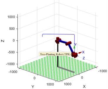
Fig. 1Self-propelled automatic poplar TPM

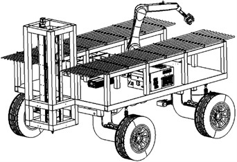
a) Axonometric view

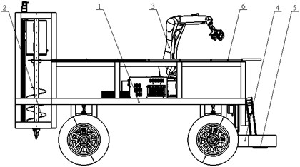
b) Main view

2. D-H model for kinematics solution

In this paper, a Denavit-Hartenberg (D-H) coordinate system for TPR modelling is proposed based on the D-H parametric approach, as shown in Fig. 2. The linkage parameters of the corresponding D-H model are shown in Table 1, where, $a_1$ = 25 mm, $a_2$ = 560 mm, $a_3$ = 35 mm, $d_4$ = 515 mm. ${\theta }_i$ represents the joint angle variable of each joint of TPR, ${\alpha }_i$ indicates the joint torsion angle, $a_{i-1}$ denotes the length of the link rod, $d_i$ is the offset of the link rod.

Using the modified D-H model coordinate transformation [8-10], the transformation expression is written as Eq. (1):

Fig. 2D-H coordinate system of a TPR

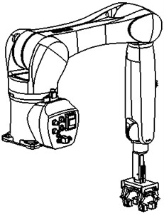
a) Axonometric view

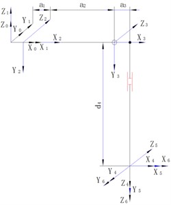
b) D-H coordinate system

The coordinate system is transformed according to the modified D-H transformation order, and the connecting rod parameters in Table 1 are substituted into Eq. (1) to obtain the flush transformation matrix ${}_1{}^0\mathrm{}T$, ${}_2{}^1\mathrm{}T$, ${}_3{}^2\mathrm{}T$, ${}_4{}^3\mathrm{}T$, ${}_5{}^4\mathrm{}T$, ${}_6{}^5\mathrm{}T$. Multiplying the above matrices from left to right, the forward motion equation of the TPR is expressed as Eq. (2) [11-13]:

where:

3. Trajectory planning analysis for TPM

In this paper, the linear interpolation of the parabolic transition is used to study the TPR trajectory planning of the TPM in the Cartesian coordinate system and the joint coordinate system, and through the numerical verification of MATLAB, the simulation results in the two coordinate systems are compared and analyzed, and the planning method is selected and evaluated.

Considering that the coordinate system 6 is located at the intersection of the 4th, 5th, and 6th axes of the manipulator, it is convenient to simplify, and the end effector of the manipulator is established in the coordinate system C, as shown in Fig. 3. The position transformation matrix of coordinate system C under coordinate system 6 is deduced.

Fig. 3Diagram of relationship between end effector in coordinate systems C and 6

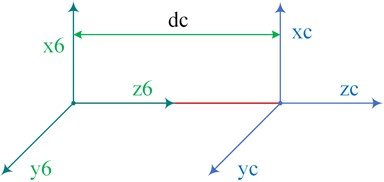
In Fig. 3, the posture of the coordinate system C of the end effector of the TPM manipulator is set to be consistent with the posture of the coordinate system 6. The position moment of coordinate system C under coordinate system 6 is written as [22]:

where, $dc$ is the distance between coordinate system 6 and coordinate system C in the direction of the $Z$-axis, the value of which is shown as $dc=$ 322.93 mm.

The starting point $P_0$, the ending point $P_f$ and the three intermediate points $P_1$, $P_2$ and $P_3$ of the TPR end-effector in the planned path are marked out, and the position and pose of each of these points and the moment of each point are planned under the base coordinate system 0 of TPR. The numerical simulation analysis data is shown in Table 2.

Table 2Position component of coordinate systems C relative to 0 at each point on the path

Track points	Time (s)	$X$ (mm)	$Y$ (mm)	$Z$ (mm)	${\varphi }_x$ ()	${\varphi }_y$ ()	${\varphi }_z$ ()
$P_0$	0	897.5	0	85	–90	0	–90
$P_1$	5	897.5	0	200	–90	0	–90
$P_2$	15	0	1238	500	0	0	0
$P_3$	20	0	1238	380	0	–90	0
$P_f$	30	0	1238	–370	0	–90	0

3.1. Trajectory planning in Cartesian coordinate system

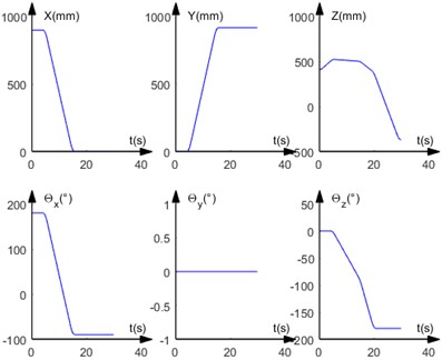
The position components of coordinate system 6 relative to coordinate system 0 at each point of the path were found using the “$XYZ$” transformation sequence according to Table 2 and ${}_6{}^0\mathrm{}{T}_i={}_C{}^0\mathrm{}{T}_i{}_C{}^6\mathrm{}{T}^{-1}$$(i=0~f)$, as shown in Table 3. Setting the acceleration time of the parabolic transition section, solving for the velocity and acceleration of the attitude components at each point, the trajectory is simulated in MATLAB as shown in Fig. 4.

Table 3Positional components of coordinate systems 6 with respect to 0 at each point of the path

Track points	Time (s)	$X$ (mm)	$Y$ (mm)	$Z$ (mm)	${\varphi }_x$ ()	${\varphi }_y$ ()	${\varphi }_z$ ()
$P_0$	0	897.5	0	407.93	180	0	0
$P_1$	5	897.5	0	522.93	180	0	0
$P_2$	15	0	915.07	500	–90	0	–90
$P_3$	20	0	915.07	380	–90	0	–180
$P_f$	30	0	915.07	–370	–90	0	–180

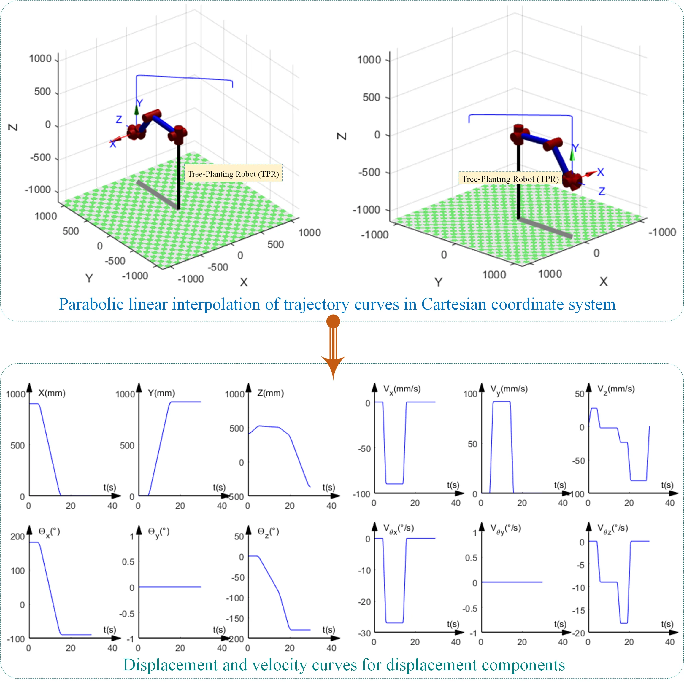
Fig. 4Parabolic linear interpolation of trajectory curves in Cartesian coordinate system

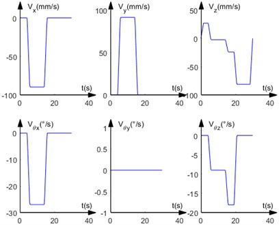
With the above planning method, the displacement and velocity profiles of the position component of coordinate system 6 with respect to coordinate system 0 and the angular displacement profiles of the six joints are shown in Fig. 5 and Fig. 6 respectively.

Fig. 5Displacement and velocity curves for displacement components

3.2. Trajectory planning in Joint coordinate system

According to the path points set in Table 2 for trajectory planning in the joint coordinate system, the kinematic inverse solution of the poses of the points in Table 2 is carried out to obtain the six joint angle values of the manipulator at each path point to, as shown in Table 4.

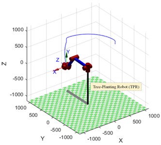
Setting the acceleration time $t_a=$ 1.5 s for the parabolic transition section, the velocities and accelerations of the six joint angles were solved for and the motion trajectory is simulated in MATLAB as shown in Fig. 7.

Fig. 6Angular displacement curve of six joints

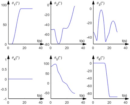
Table 4Six joint angle values of the manipulator at each path point

Track points	Time(s)	${\theta }_1$ ($°$)	${\theta }_2$ ($°$)	${\theta }_3$ ($°$)	${\theta }_4$ ($°$)	${\theta }_5$ ($°$)	${\theta }_6$ ($°$)
$P_0$	0	0	–50.4138	–33.0731	0	83.4868	0
$P_1$	5	0	–49.2030	–47.9657	0	97.1687	0
$P_2$	15	90	–47.0087	–49.1878	0	6.1965	0
$P_3$	20	90	–47.9434	–34.1929	0	–7.8638	–90
$P_f$	30	90	–2.6970	–33.2546	0	–54.0484	–90

Fig. 7Parabolic linear interpolation trajectory curves in the joint coordinate system

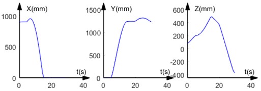
The angular displacement and angular velocity curves for the six joints under this planning method and the three displacement component curves for the origin of the coordinate system C under the Cartesian coordinate system are shown in Fig. 8 and Fig. 9 respectively.

By comparing Fig. 4 and Fig. 7, it can be seen that when the trajectory planning method with parabolic transition linear interpolation is used for trajectory planning in a right-angle coordinate system, the trajectory at the end of the robot arm basically consists of straight-line segments and parabolic segments, and its trajectory matches the path planned at the beginning. When the trajectory planning method is used for trajectory planning in the joint coordinate system, the trajectory at the end of the robot arm basically consists of parabolic and some straight-line segments, and its final trajectory is different from the path planned at the beginning.

Poplar saplings avoid the platen in the compaction mechanism during the planting process, so that the saplings can be put into the pit more smoothly through the reserved gap in the platen. TPM uses parabolic transition linear interpolation in the joint coordinate system for trajectory planning. This planning method significantly reduces the amount of manipulation of the manipulator during the tree planting process. Under the planning method, the angular displacement of the six joints of the manipulator varies linearly, which effectively avoids the creation of odd shapes of the manipulator.

Fig. 8Angular displacement and angular velocity curve of six joints

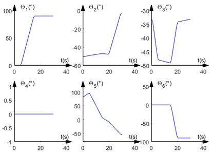
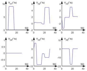
Fig. 9Displacement component curve of the end-effector

4. Conclusions

This paper proposes an improved D-H parameter method, analyzes the mathematical model of the actuator TPR in the TPM, solves the forward kinematic equation of the manipulator in the TPR by matrix transformation, and deduces the joints of the manipulator by using the separation of variables method. Inverse numerical solution. A linear programming method based on parabolic transition is used to plan the motion trajectory in Cartesian coordinate system and joint coordinate system. By comparing the planning results in the two coordinate systems, considering the structural characteristics of TPM, an appropriate planning method is selected, which provides a theoretical basis for the subsequent tree planting process of TPM.

This paper addresses some of the research in inverse kinematics and path planning for TPRs, breaking through the limitations of industrial robots concentrated in unconstrained workspaces with homogeneous objects, and successfully combining the capabilities of TPRs with the environment in which it operates in forests. Tree planting environments are known to be complex.