Frequency monitoring analysis of milling edge chatter in composites using WPD for frequency band selection

1. Introduction

Higher standards for the various material qualities are imposed by the advancement of aeronautical technology. And composite materials, which are made of two or more different substances combined in various ways, overcome the flaws of a single material. They are frequently used in the production of solar cell wings and shells, large launch vehicle shells, aircraft wings, satellite antennas, engine shells, and structural components of spacecraft, among other things. It is extremely challenging to manufacture and especially prone to chattering because of the varied properties of the layers of material used in the machining process. Chattering can readily reduce the workpiece's quality by, for instance, increasing surface roughness and decreasing precision. Additionally, it causes the system to become unstable, which accelerates the deterioration of tool and machine life and raises production costs [1, 2]. Because of this, controlling and reducing chatter generation has become a significant challenge in the processing of composite materials today. The analysis of the system's stability using a dynamical model yields a stability leaflet diagram, from which the maximum milling depth and the key circumstances for system stability may be computed. This is one of the two primary ways to chatter monitoring. The alternative method is to monitor the chattering signal using empirical mode decomposition (EMD). But the initial frequency of chatter is not visible and is easily covered by the background noise, and other frequency bands are not sensitive to chatter [3, 4]. As a result, chatter monitoring is not very accurate. There are instances of leakage and misjudgment, which together with the fact that the majority of existing research concentrate on a single signal further diminish the monitoring accuracy. The research suggests a chattering frequency monitoring technique based on the Frequency Elimination Algorithm (FEA) and Wavelet Packet Decomposition (WPD). Compared to the conventional filtering technique, this approach efficiently eliminates insignificant signals, extracts the flutter-sensitive frequency band, removes abnormal characteristic points, and establishes the flutter monitoring threshold.

The study is broken into four parts: the first part gives a quick summary of the state-of-the-art in chatter monitoring and WPD research; the second part examines FEA and WPD; the third part examines FEA and WPD; and the fourth part examines FEA and WPD. The third part analyses the experimental data; and the fourth and final section provides a summary of the entire body of work.

2. Related works

Li Y. and his team propose an adaptive decision tree and variational mode decomposition based chatter identification method for the monitoring of chatter. The process uses a decision tree to calculate the chattering threshold after adaptive variational mode decomposition divides the original signal into many sub-signals. The results of the experiments demonstrated that the approach can accurately and successfully identify chatter [5]. Jin et al. proposed a stability prediction method based on a dynamics model. By creating a dynamics model of the thin-walled workpiece milling system and employing a numerical integration approach to produce the milling system's stability waveform diagram, the method determines the chattering frequency. The tested method's experimental results and the anticipated outcomes agree rather well [6]. Rahimi et al. have proposed a chatter monitoring method based on machine learning algorithms and physical models for the detection of milling vibrations. The method converts the vibration signal into a short-time spectrum and enhances the chattering signal by Kalman filtering. According to the experimental findings, the approach for chatter detection had a success rate of up to 98.9 % [7]. To solve the issue of how to automatically alter the chatter threshold, Stavropoulos P and others suggested a chatter detection system based on variational mode decomposition and support vector machines. The method decomposes the vibration signal to extract features in different simultaneous frequency domains and uses support vector machines to make predictions about system stability. The method was tested to achieve a classification accuracy of 93 % and a detection time of only 26.1 ms [8]. In order to quickly and correctly detect chatter, Gao and his team suggested a multi-sensor signal fusion-based chatter detection approach. The approach uses variable modal decomposition energy entropy, multi-scale power spectrum entropy, and multi-scale displacement entropy to interpret the signals gathered by various sensors. The experimental findings demonstrated the method's accuracy in detecting the milling machining state [9].

As a time-frequency domain analysis method, WPD is widely used for processing various types of signals because it can describe the signal characteristics very accurately. To solve the issue of how to perform the denoising of noisy signals from automobiles, Liang L. et al. suggested a signal extraction approach based on WPD and mathematical morphological filters. According to experimental findings, the approach effectively removed interfering background noise from the signal and extracted the components of the tapping sound with a decent signal-to-noise ratio [10]. Wang and others have proposed a fault detection model based on WPD and BiCNN to address the problem of how to achieve fault detection in the presence of data imbalance. In order to counteract the negative effects of data scarcity, the model uses WPD to mine data across a variety of frequency domains. The model has been tested to have good classification performance in the presence of data imbalance [11]. Hossen and Qasim proposed a WPD and ANN based identification model for the problem of how to identify obstructive sleep apnoea. The model uses WPD to obtain and estimate the standard band of HRV signals and ANN to classify test subjects. The experimental results showed that the model achieved 95 % accuracy in classifying negative normal subjects and mild OSA subjects, and 87.5 % accuracy in classifying mild, moderate and severe OSA subjects [12]. Fan X. B. and his team proposed a WPD-based analysis method to address the problem of how to analyse non-stationary signals; the method decomposes the original signal by WPD and reconstructed by WPD. The technique outperformed the competition in the analysis of non-stationary signals, according to experimental results [13]. For the fault detection issue of the mix production process, Chen Y. et al. suggested a fault detection model based on WPD and SVM. The model extracts features by wavelet basis functions and classifies faults by using SVM. The fault detection accuracy of the model was tested to be 4.33 % higher than that of PCA [14].

In summary, the research on chattering frequency monitoring models has been quite successful, but most of the methods are not effective in monitoring the frequency at the beginning of chattering because the frequency at the beginning of chattering is masked by the spindle rotation frequency, etc. To address this problem, a chattering frequency monitoring algorithm based on FEA and WPD is proposed to achieve accurate monitoring of chattering frequency.

3. Frequency monitoring method for milling edge chatter in composites based on FEA and WPD algorithms

In the field of aerospace manufacturing, the monitoring and suppression of milling edge chatter in composite materials has been a difficult research problem, especially since the milling edge processing process is often accompanied by changes in the signal spectrum and band energy ratio distribution, which exacerbates the monitoring difficulty. In order to realise the frequency monitoring of milling edge chatter, a frequency monitoring method based on FEA and WPD algorithms is proposed.

3.1. FEA research

Since the initial frequencies of the chatter are not obvious, and the frequency signal often contains spindle rotations and multipliers unrelated to the chatter, making it difficult to extract the relevant signal, the irrelevant signal must be removed. The traditional filters can often only remove a single frequency and cannot achieve the removal of multiple frequencies [15]. To solve the above problem, research proposed FEA based on FFT. FFT as a kind of discrete Fourier transform algorithm, its solve the traditional discrete Fourier algorithm of the computational shortcomings of the large amount. Compared with the traditional filtering method, this method can effectively remove irrelevant signals and extract the flutter sensitive frequency band, and eliminate the abnormal characteristic points and determine the flutter monitoring threshold. Now suppose there is a sequence, then the Fourier transform equation of the sequence is shown in Eq. (1):

1

$X\left(k\right)=\sum _{r=0}^{N/2-1}{x}_1\left(r\right)W_N^{2kr}+W_N^k\sum _{r=0}^{N/2-1}{x}_2\left(r\right)W_N^{2kr}=\sum _{n=o\mathrm{d}\mathrm{d}}x\left(n\right)W_N^{kn}+\sum _{n=\mathrm{e}\mathrm{v}\mathrm{e}\mathrm{n}}x\left(n\right)W_N^{kn},$

where, $x\left(n\right)$ denotes the sequence; $W_N^m$ denotes the rotation factor; $N$ denotes the length of the sequence; $x_1\left(r\right)$ and $x_2\left(r\right)$ denote the subsequence of length $N/2$ divided by the parity of $n$. The equation for the subsequence and the rotation factor are given in Eq. (2):

2

$W_N^{2kr}=e^{-j\frac{2\pi }{N}2kr}=e^{-j\frac{2\pi }{N/2}kr}=W_{N/2}^{kr}.$

Substitute the above equation into Eq. (1) to obtain Eq. (3):

3

$X\left(k\right)=\sum _{r=0}^{N/2-1}{x}_1\left(r\right)W_{N/2}^{kr}+W_N^k\sum _{r=0}^{N/2-1}{x}_2\left(r\right)W_{N/2}^{kr}=X_1\left(k\right)+W_N^k{X}_2\left(k\right),$
$k=\mathrm{0,1},\cdots ,N-1,$

where, $X_1\left(k\right)$ and $X_2\left(k\right)$denote $N/2$ odd sequence points and even sequence points, respectively, both with period $N/2$; $W_N^{k+N/2}=-W_N^k$. Thus Eq. (3) can be rewritten as Eq. (4):

4

$\left\{\begin{array}{ll}X\left(k+N/2\right)=X_1\left(k\right)-W_N^k{X}_2\left(k\right),& k=\mathrm{0,1},\cdots ,\frac{N}{2}-1,\\ X\left(k\right)=X_1\left(k\right)+W_N^k{X}_2\left(k\right),& k=\mathrm{0,1},\cdots ,\frac{N}{2}-1.\end{array}\right.$

Eq. (4) is known as the butterfly operation. When the sequence length is 8, the butterfly calculation flow is shown in Fig. 1.

Fig. 1Butterfly calculation process for 8 points

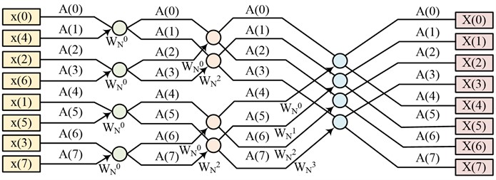
As can be seen in Fig. 1, the butterfly calculation of eight points is divided into three stages, which first perform the calculation of two points, before merging to four points and performing the calculation again. The computation time of this method is halved compared to the conventional discrete Fourier transform [16-17]. The system chatter will generate a non-periodic component during the machining operation of the machine tool, and this component will gradually approach the natural frequency of the machine tool. At the same time, the initial frequency amplitude is very small, so it is masked by the rotational frequency and difficult to detect, so the spindle rotational frequency and multiplication frequency must be eliminated by FEA. The equation for calculating the spectrum of the time series is shown in Eq. (5):

5

$\left\{\begin{array}{l}X\left(i\right)=\sum _{k=1}^{M}x\left(k\right)W_M^{ki},\mathrm{}\mathrm{}\mathrm{}\mathrm{}\mathrm{}k=\mathrm{1,2},\cdots ,M,\\ W_M=\mathrm{e}\mathrm{x}\mathrm{p}\left(-j\frac{2\pi }{M}\right),\end{array}\right.$

where, $X\left(i\right)$ denotes the spectrum obtained from the time series transformation; $M$ denotes the length of the spectrum, units in s; $x\left(k\right)$ denotes the time series. The equation for calculating the spindle rotation frequency and multiplication frequency is shown in Eq. (6):

6

$\left\{\begin{array}{l}{f}_z=\frac{n_s}{60},\\ f_d=c{f}_z,\end{array}\right.$

where, $f_z$ indicates the spindle frequency, units in Hz; $n_s$ indicates the spindle speed, units in r/min; $f_d$ indicates the multiplier frequency, units in Hz; $c$ indicates the initial value. The equation for calculating the spectrum considering the fluctuation of the transformation frequency is shown in Eq. (7):

7

$\stackrel{-}{X}\left(i\right)=\left\{\begin{array}{ll}0,& c{f}_z-a\le i\le c{f}_z+a,\\ X\left(i\right),& \left(c-1\right)f_z+a\le i\le c{f}_z-a,\end{array}\right.$

where, $a$ denotes the floating constant and takes the value of 0.5, $\stackrel{-}{X}\left(i\right)$ represents the frequency spectrum after the interval amplitude of the frequency $\left(f_z-a,f_z+a\right)$. The equation for calculating the time series after the inverse Fourier transform is given in Eq. (8):

8

$x\left(k\right)=\sum _{i=1}^M\stackrel{-}{X}\left(i\right)W_M^{-ki},\mathrm{}\mathrm{}\mathrm{}\mathrm{}\mathrm{}k=\mathrm{1,2},\cdots ,M,$

where, $x\left(k\right)$ denotes the inverse Fourier transformed time series. The FEA process is shown in Fig. 2.

Fig. 2Flow of FEA

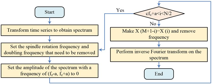
As can be seen from Fig. 2, FEA will first transform the time series to obtain the spectrum; after obtaining the spectrum, remove the spindle transconversion and multiplication; then set the spectrum amplitude of frequency $(f_z-a,f_z+a)$ in the spectrum to 0, if $c{f}_z<i<N/2$, then return to the second step; otherwise proceed to the next step to de-frequency the spectrum.

3.2. Research on WPD-based SFB selection algorithm

The signal spectrum is often very complex and it is difficult to extract the chatter characteristics accurately. Calculations are also complicated by the different sensitivities of different frequency bands. It is therefore necessary to accurately identify the chatter sensitivity bands in order to monitor the chatter frequency. The WPD equation and the band reconstruction equation are given in Eq. (9):

9

$\left\{\begin{array}{l}{d}_{n+\mathrm{1,2}j}^l={\sum }_k{a}_{k-2l}{d}_{n,j}^k,\\ d_{n+\mathrm{1,2}j+1}^l={\sum }_k{b}_{k-2l}{d}_{n,j}^k,\\ d_{n+1,j}^k={\sum }_l{a}_{2k-l}{d}_{n+\mathrm{1,2}j}^l+{\sum }_l{b}_{2k-l}{d}_{n+\mathrm{1,2}j+1}^l,\end{array}\right.$

where, $d$ denotes the WPD coefficient; $a$ denotes the high-pass filtering coefficient; $b$ denotes the low-pass filtering coefficient; $n$ denotes the number of decomposition layers; $j$ denotes the band node number; and $k$ denotes the number of bands. the WPD structure is shown in Fig. 3.

Fig. 3Structure of WPD

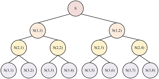
As shown in Fig. 3, the WPD divides the signal into high frequency and low frequency components after signal acquisition. The signal is then divided again, and so on, until the decomposition is complete. The frequency case of the WPD decomposed signal is ordered by the Gray code law [10, 19, 20]. In the system frequency band energy ratio, energy entropy as its characteristic quantity is often used to reflect the change of the frequency band energy ratio. The energy entropy calculation equation is shown in Eq. (10):

10

$\left\{\begin{array}{l}{P}_i=\frac{E_i}{E},\\ H=-\sum _{i=1}^N{P}_i\mathrm{l}\mathrm{o}{\mathrm{g}}_2\left|P_i\right|,\end{array}\right.$

where, $P_i$ denotes the normalised $i$th band energy ratio; $E_i$ denotes the $i$th band energy, units in mV.s; $E$ denotes the energy of all bands; $H$ denotes the energy entropy; and $N$ denotes the number of bands. The band energy ratio determines the sensitivity of the energy entropy value to chattering, and the correlation coefficient and the fluctuation variance of the band energy ratio can be used to select the frequency bands with stronger sensitivity to chattering, so as to improve the performance of the energy entropy in identifying the initial frequency of chattering. The correlation coefficient is given in Eq. (11):

11

$\left\{\begin{array}{l}\rho \left(s_i,S\right)=\frac{\mathrm{c}\mathrm{o}\mathrm{v}\left(s_i,S\right)}{\sqrt{D\left(s_i\right)D\left(S\right)}},\mathrm{}\mathrm{}\mathrm{}\mathrm{}\mathrm{}i=\mathrm{1,2},\cdots 2^n,\\ D\left(s_i\right)=\frac{\sum _{t=1}^T{\left(s_i\left(t\right)-\stackrel{-}{s}\right)}^2}{T},\\ D\left(S\right)=\frac{\sum _{t=0}^T{\left(S\left(t\right)-\stackrel{-}{S}\right)}^2}{T},\end{array}\right.$

where, $\rho \left(s_i,S\right)$ denotes the correlation coefficient; $s_i$ denotes the $i$th band reconstruction signal; $S$ denotes the original signal; $D\left(S\right)$ denotes the covariance of the raw signal; $\mathrm{c}\mathrm{o}\mathrm{v}\left(s_i,S\right)$ denotes the covariance between the band reconstruction signal and the original signal; $n$ denotes the number of WPD layers; $\stackrel{-}{s}$ denotes the mean of the band reconstruction signal; $S$ denotes the mean of the original signal; $D\left(s_i\right)$ denotes the variance of the band reconstruction signal; $T$ denotes the sampling period, units in s; $s_i\left(t\right)$ denotes the covariance of the band reconstruction signal within the $t$ moment; $S\left(t\right)$ denotes the original signal within the EE moment E denotes the original signal at the time of $t$. When $\left|\rho \left(s_i,S\right)\right|\le 0.1$, the band reconstruction signal is weakly correlated with the original signal; when $0.1<\rho \left(s_i,S\right)\le 0.5$, the band reconstruction signal is correlated with the original signal; when $0.5<\rho \left(s_i,S\right)\le 1$, the band reconstruction signal is strongly correlated with the original signal. The stronger the correlation between the band and the original signal and the more accurate information in the signal, or the opposite, the more interfering signals, the larger the correlation coefficient between the band reconstructed signal and the original signal. In the steady state, the band energy ratio fluctuations during the sampling period are normally distributed. When dither occurs, the band energy fluctuates dramatically and gradually converges to the intrinsic frequency, so the sensitivity of the reconstructed signal to dither anomalies can be reflected by the band energy ratio fluctuation variance. The band energy ratio fluctuation variance is calculated by Eq. (12):

12

${\sigma }_i\left(t\right)=\frac{\sum _{t=0}^T{\left(P_i\left(t\right)-{\mu }_i\right)}^2}{T},\mathrm{}\mathrm{}\mathrm{}\mathrm{}\mathrm{}i=\mathrm{1,2},\cdots ,N,$

where, ${\sigma }_i{\left(t\right)}^2$ denotes the fluctuating square of the band energy ratio; ${\mu }_i$ denotes the average value of the energy ratio of the first band; $P_i\left(t\right)$ denotes the energy ratio of the $i$ th band at the $t$ moment. The greater the difference between the band energy ratio fluctuation square, the more sensitive the band is to chattering, otherwise it means the band is not sensitive to chattering. If the energy ratio is greater than 0.13, the frequency band has high sensitivity, whereas if the ratio is less than this threshold, the sensitivity is low. Eliminating the interference of the less sensitive bands based on the band's correlation with the original signal and the energy ratio fluctuation is important to increase the sensitivity of the characteristic quantity to the initial frequency monitoring of dither. The conditions to be satisfied for the dither SFB are shown in Eq. (13):

13

$\left\{\begin{array}{l}\rho >\left[\rho \right],\\ \left\{{\sigma }^2\right\}=\left\{\begin{array}{ll}{\sigma }_1^2,{\sigma }_2^2,\cdots ,{\sigma }_j^2& j=\mathrm{1,2},\cdots ,N_i\end{array}\right\},\end{array}\right.$

where ${{\sigma }_j}^2$ stands for the energy ratio fluctuation variance in the $j$th band. Eq. (14), which describes the $N_i$ formula:

14

$N_i=round\left(a\cdot N\right),$

where, $N$ denotes the number of bands after WPD; “round” denotes the rounding function in Matlab; and $a$ denotes the sensitivity factor. The SFB logic is shown in Fig. 4.

Fig. 4Sensitive frequency band logic

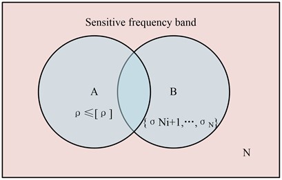
As shown in Fig. 4, the band is SFB when both conditions described in Eq. (13) are satisfied, and the equation is expressed in Eq. (15):

15

$s_i=\overline{A\cup B},$

where, $A$ denotes the band that satisfies $\rho \le \left[\rho \right]$; $B$ denotes the band where the variance of the energy fluctuation ratio lies after $N_i$.

4. Experimental results and analysis

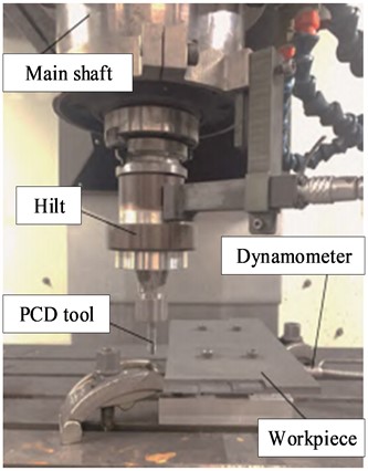
Experiments on FEA and WPD are conducted in order to validate the efficacy of the chattering frequency monitoring approach suggested in the study. In the validation experiments on FEA, the performance of its frequency cancellation will be tested by synthesising the signal. In the validation experiments for WPD, the performance of its frequency monitoring will be verified using signals acquired during machining and compared with EMD. The material size used for machining is 300 mm×140 mm×6.5 mm and the tool diameter is 8 mm; and the milling force signal in the feed direction at different milling edge depths is measured using a force gauge, the meter is Kistler 9257B; the sensor’s sample frequency is set at 10 kHz. The feed rate is 120 mm/s, and the spindle speed is 4000 r/min. The experimental processing apparatus is shown in Fig. 5.

Fig. 5Experimental processing device

The relevant data including the milling edge depth of the experiment are shown in Table 1.

Fig. 6 displays the initial synthesised signal as well as the signal following de-frequencying.

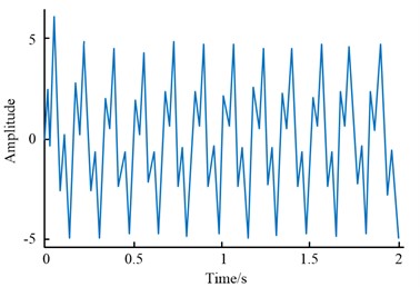
The original signal, which has an amplitude maximum at 10, is more chaotic and without any discernible pattern, as shown in Fig. 6(a). As shown in Fig. 6(b), the signal essentially exhibits periodic changes following the FEA de-frequency, with the exception of the initial phase of the signal, which exhibits a subtle Gibbs phenomenon. In addition, the maximum amplitude value also decreases from 10 to about 5. This shows that the FEA has more completely restored the signal to be preserved. The signal spectrum and its de-frequency results are shown in Fig. 7.

Fig. 7(a) shows that the original signal has the following frequencies: 6, 18, 40, 80, 120, 160, and 200 Hz, where 40, 80, 120, 160, and 200 Hz all have an amplitude of roughly 1. The de-frequency signal only has two frequencies, 6 Hz and 18 Hz, which are represented by amplitudes of about 2.9 and 2, respectively, as can be seen in Fig. 7(b). The above results show that the FEA algorithm has excellent frequency cancellation capability and can accurately remove a certain fundamental frequency and its multiples. The processed signals and their de-frequency results are shown in Fig. 8.

Fig. 6Original synthesized signal and signal after frequency reduction

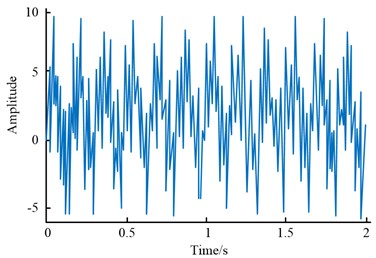
a) Raw synthetic signal

b) Signal after frequency reduction

Fig. 7Signal spectrum and its frequency reduction results

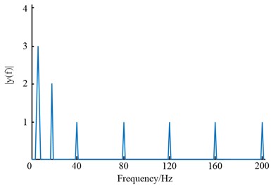
a) The spectrum of the original synthesized signal

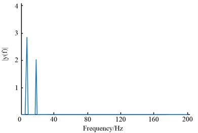
b) Signal spectrum after frequency reduction

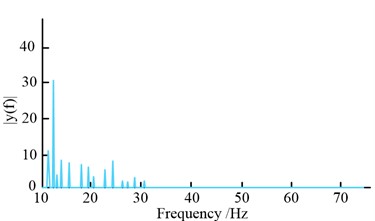
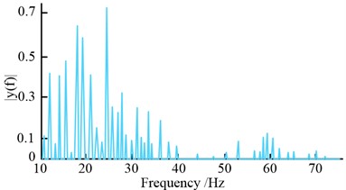
Figure 8(a) illustrates how the milling force increases incrementally as the milling depth increases. A milling depth of 0.5 mm results in a force of about 10 N; a depth of 2 mm results in a force of about 51 N; a depth of 4 mm results in a force of about 120 N; and a depth of 6.5 mm results in a force of about 162 N. As can be seen from Fig. 8(b), the spindle rotation frequency and the DC component are more prominent in the signal spectrum of the original signal and are concentrated mainly in the low frequency. The spindle frequency is about 66.7 Hz and the corresponding amplitude is about 12.7, while the tooth frequency of the cutter tooth is about 133.4 Hz and the corresponding amplitude is about 32.8. The above signals mask the chattering signal, which makes it difficult to be detected, so the frequency cancellation of the original signal is needed. In Fig. 8(c), the signal after de-frequency fluctuates more at the junction where the milling edge depth changes. For example, when the tool is located at the junction of 0.5 mm^-2 mm, the milling force first rises rapidly to about 20 N and then drops sharply to about 10 N. This is because the feed to the tool teeth increases suddenly at this point, which breaks the original equilibrium and intensifies the fluctuation of the milling force; therefore, the system is prone to chattering phenomenon. As can be seen from Fig. 8(d), the chattering frequency is very easy to observe in the signal spectrum after the de-frequency, and the chattering frequency is about 1333 Hz at this time. The WPD is required to estimate the dither signal's production time because, despite the fact that the aforementioned approach can identify the dither signal, doing so is challenging. The correlation coefficients, energy ratio variance and sensitivity bands for each frequency band after de-frequency are shown in Fig. 9.

Fig. 8Processing signal and its frequency reduction results

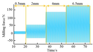
a) Original signal

b) Raw signal spectrum

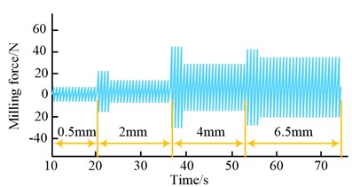
c) Signal after frequency reduction

d) Signal spectrum after frequency reduction

Fig. 9Correlation coefficient, energy ratio variance, and sensitivity band of each frequency band after frequency reduction

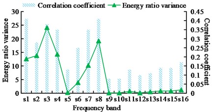
a) Correlation coefficients and energy variance of each frequency band after frequency reduction

b) Comparison of strong and weak sensitive zone

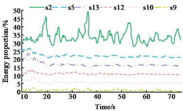
From Fig. 9(a), the correlation coefficients of frequency bands s1-s16 after de-frequency are about 0.41, 0.28, 0.38, 0.35, 0.13, 0.25, 0.35, 0.41, 0.08, 0.08, 0.13, 0.1, 0.11, 0.14, 0.14 and 0.17 respectively; the energy ratio variances are about 12.6, 13.8, The correlation coefficients of s9, s10, s12 and s13 are small, and the energy ratio variances of s5, s9, s10, s11, s12 and s13 are in the latter 31.25% of all bands, all of which are insensitive to chattering. Fig. 9(b) shows that at a time of 37 s, the energy ratio of band s2 is at its maximum point, around 49%, while the energy ratios of bands s5, s9, s10, s12, and s13 are all at their lowest points, respectively, at 23 %, 0.9 %, 5 %, 10 %, and 16 %, all of which exhibit a modest sensitivity to dither. It can be seen that if the sensitivity of chatter monitoring is to be improved, the above-mentioned frequency bands should not be taken into account when calculating the energy entropy. The energy entropy for different milling edge depths is shown in Fig. 10.

As can be seen from Fig. 10(a), when the milling depth is 0.5 mm, the energy entropy fluctuates at 15,000 and 80,000 points, where the energy entropy is 3.3 and 3.1 respectively; at around 70,000 points, the energy entropy reaches its maximum, at around 3.7. The energy entropy reaches its lowest and maximum peaks at 40,000 and 70,000 points, respectively, when the milling edge depth is 2 mm, as shown in Fig. 10(b). The corresponding energy entropies are 2.7 and 3.5 respectively and fluctuate rapidly at 40,000 points. The energy entropy fluctuates more at 41000 and 70000 points with corresponding energy entropies of 2.6 and 3.6 as shown in Fig. 10(c) when the milling depth is 4 mm. This is due to the fact that the actual machining process is extremely contingent and therefore the energy entropy does not exactly follow a normal distribution. The chatter thresholds for different milling depths are shown in Fig. 11.

Fig. 10Energy entropy of different milling depths

a) Milling depth 0.5 mm

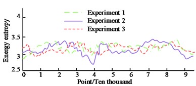
b) Milling depth 2 mm

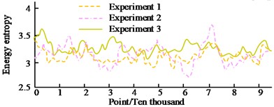
c) Milling depth 4 mm

Fig. 11Flutter thresholds for different milling depths

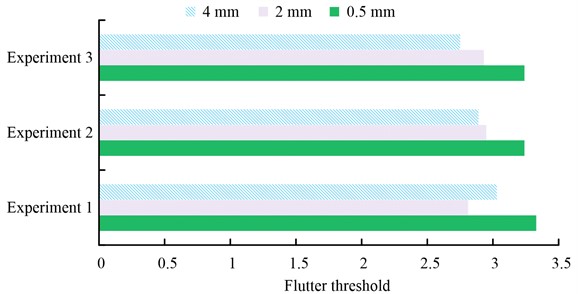
As can be seen from Fig. 10, the chatter thresholds for the three experiments were 3.33, 3.24 and 3.24 for a milling depth of 0.5 mm, with an average threshold of about 3.27; for a milling depth of 2 mm, the chatter thresholds were 2.81, 2.95 and 2.93 for the three experiments, with an average threshold of 2.9; for a milling depth of 4 mm, the chatter thresholds were 3.03, 2.89 and 2.75 for the three experiments, with an average threshold of about 2.89. The above results show that the chatter threshold decreases as the milling depth increases. This is as a result of the system's instability increasing with increasing milling depth. The energy entropy values at the junction of the milling edge depth after de-frequency are shown in Fig. 12.

Fig. 12 shows that the energy entropy of the original signal fluctuates strongly at the intersection of the milling depths of 0.5 mm, 2 mm and 4 mm, where the energy entropy is about 3 and 2.4 respectively. However, at the intersection of the milling depths of 4 mm and 6 mm, the fluctuation is not obvious and it is difficult to identify the abnormal signal; the average energy entropy is about 1.05. The average energy entropy of the signal after de-frequencying is about 3.2, and at the junction of the milling depths, the energy entropy is about 2.8, 2.6 and 2.65 respectively, which are lower than the respective dither thresholds and can obviously detect the abnormal signal. The energy entropy of WPD and EMD is shown in Fig. 13.

Fig. 12Energy entropy value at the junction of milling depth after frequency reduction

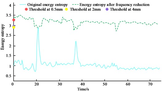
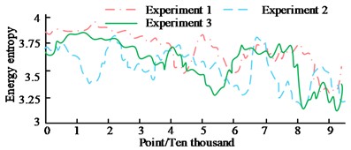
Fig. 13Characteristics of flutter signals for WPD and EMD

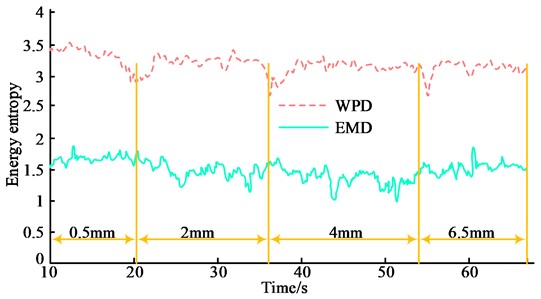
Fig. 13 displays that the energy entropy of the chattering signal produced by the EMD has an average value of approximately 1.55. However, its variation at the milling edge depth junction is not immediately apparent. This lack of clarity makes it difficult to identify system chattering. The insensitivity of the EMS to chattering frequency changes at the initial stage is the primary cause of this issue. The energy entropy of the WPD varies substantially and distinctly at the junction of the milling edge depth for energy entropy levels around 2.9, 2.6 and 2.5, respectively. This is when the chattering phenomenon becomes clearly detectable, demonstrating the WPD’s increased sensitivity to chatter frequency monitoring.

5. Conclusions

Due to the variance in milling edge depth, the system is vulnerable to chattering throughout the milling operation. The paper suggests a WPD-based chatter frequency monitoring technique to accomplish reliable chatter signal frequency monitoring. The process uses WPD to track the chatter frequency and FEA to filter out extraneous signals from the original machining signal. Separate tests of the FEA and WPD revealed that the signal only contained two frequencies, 6 Hz and 18 Hz, as opposed to the original signal's de-frequencying, which eliminated the undesirable signal. The original machining signal's spindle rotation frequency and DC component can obscure the dither frequency, making it challenging to detect, but the de-frequencyed machining signal swings more at the point where the milling edge depth changes. For instance, the milling force increased quickly to about 20 N and then dramatically decreased to about 10 N when the tool was at the 0.5 mm-2 mm junction. The energy ratio variances for s5, s9, s10, s11, s12, and s13 were in the bottom 31.25 % of all bands. The correlation coefficients for s9, s10, s12, and s13 in the de-frequency band were minimal, at 0.08, 0.08, 0.1, and 0.11 correspondingly. The influence of the aforementioned bands should be avoided while computing the energy entropy because they are all insensitive to chattering. At the intersection of the milling edge depth, where the energy entropy was around 2.8, 2.6, and 2.65, respectively, the de-frequency signals exhibit abrupt variations that were easily distinguishable from normal signals since they are all below the corresponding dither thresholds. Contrarily, the energy entropy of the EMD chatter signal averaged around 1.55, but its variation at the intersection of the milling edge depth was not noticeable, making it challenging to detect the chatter of the system. The aforementioned findings demonstrated that the WPD and FEA-based chatter monitoring techniques are more sensitive.