An assembled hot wire anemometer design

Yao, Xingxing; Shen, Fanhao; Zheng, Yuan; Xiao, Ting

doi:10.21595/jme.2023.23637

Journal of Measurements in Engineering

Browse Journal

Submit article

Published: 03 January 2024

Check for updates

An assembled hot wire anemometer design

Xingxing Yao¹

Fanhao Shen²

Yuan Zheng³

Ting Xiao⁴

^{1, 2, 3, 4}School of Physics, Zhejiang University, Hangzhou, China

Corresponding Author:

Xingxing Yao

Cite the article Download PDF

Downloads 86

Abstract

The hot wire anemometer is a widely utilized device in laboratory settings for measuring air speed. This paper investigates the relationship between air speed and hot wire temperature across various air speed ranges, employing the theory of thermal equilibrium. We designed a measurement circuit and hot wire shape based on the hot wire anemometer principle, and validated the linear relationship between current and temperature at different air speeds within an adjustable air speed field. The measured current serves as a representative of air speed. Experimental validation of the designed hot wire anemometer demonstrates accurate measurement results that align with theoretical values across different air speed ranges. Finally, we determined the sensitivity of the anemometer in various measurement ranges, considering the instrument's uncertainty and measurement formula.

1. Introduction

The precise measurement of air speed plays a crucial role in both laboratory and engineering applications [1]. Accurate assessments are fundamental to understanding fluid dynamics, optimizing aerodynamic performance, and enhancing various industrial processes. A myriad of instruments are employed for air speed measurement, including mechanical anemometers, laser Doppler anemometers, ultrasonic anemometers, particle image velocimetry, and hot-wire anemometers [2]-[7]. Among these, hot-wire anemometers stand out due to their notable advantages: a broad measurement range, rapid measurement speed, and high sensitivity [8]. The operating principle of a hot-wire anemometer is rooted in the generation of heat when an electric current passes through a thin wire. As the wind flows over the hot wire, forced convection from the wire dissipates heat, resulting in a decrease in wire temperature and resistance. The air speed is then determined by establishing the relationship between pertinent physical quantities. This type of anemometer has gained widespread acceptance in both research and industrial applications owing to its accuracy, reliability, and operational convenience [9]-[13]. While computer simulations have been instrumental in studying the behavior of hot-wire anemometers under various conditions [14]-[17], recent advancements in the field call for attention. Scholars have delved into visualizing and analyzing scenarios involving different forms of hot wires in diverse environmental conditions [18]-[21]. Notably, Pankaj Charan Jena's work emphasizes the pivotal role of heat exchangers in various industries and underscores the need for advanced designs to meet current industrial demands [22]. The study proposes a modeling and design approach utilizing the finite element method, specifically computational fluid dynamics. ANSYS 15.0 is employed to analyze the heat transfer rate of shell and tube-type heat exchangers, incorporating vertical baffles in the design and simulation. The research contributes valuable insights into the selection of input parameters, modeling techniques, and simulation methodologies.

In the present study, we delve into the design of a multi-range anemometer, incorporating self-designed hot wires and measurement circuits. Our focus lies in optimizing design parameters to ensure measurement sensitivity while addressing the limitations observed in existing hot-wire anemometer models. By developing an innovative approach, we aim to contribute to the refinement of air speed measurement techniques, fostering advancements in fluid dynamics research and enhancing the applicability of such instruments in various scientific and industrial domains.

2. Theoretical basis

Generally, heat exchange between a heated wire and its surroundings manifests in four modes: natural convection, forced convection, heat conduction, and thermal radiation. Taking into account a scenario where the wire is subjected to external heating (e.g., electrical current) and subsequently dissipates heat through all the aforementioned mechanisms to its surroundings, the power balance equation can be articulated upon achieving thermal equilibrium in the system:

1

P_{I n p u t} = P_{F o r c e d c o n v e c t i o n} + P_{N a t u r a l c o n v e c t i o n} + P_{H e a t c o n d u c t i o n} + P_{H e a t r a d i a t i o n},

2

i^{2} R_{e} = h A_{w} (T - T_{0}) + P_{N a t u r a l C o n v e c t i o n} + P_{H e a t c o n d u c t i o n} + A_{w} σ ε (T^{4} - T_{0}^{4}) .

Because the length of the hot wire is much larger than its cross section, the heat transfer caused by conduction is negligible. For small temperature changes there is $T^{4} - T_{0}^{4} = T_{0}^{3} (T - T_{0})$ . $P_{N a t u r a l C o n v e c t i o n}$ can be considered constant. Eq. (2) is rewritten as:

3

i^{2} R_{e} = h^{'} A_{w} (T - T_{0}),

where: $A_{w}$ is the surface area of the electric heating wire; $T_{0}$ is the ambient temperature, $T$ is the temperature of the heating wire at a specific power; $σ$ is the Stefan-Boltzmann constant, $ε$ is the emissivity; $h$ is the forced convection heat conversion coefficient, $h^{'}$ is the equivalent heat conversion coefficient.

From King’s law in thermodynamics, the following equation is known when the air speed is high:

4

\frac{d H}{d t} = i^{2} R_{e} - (K + C \sqrt{V}) (T - T_{0}) .

When air speed is low:

5

\frac{d H}{d t} = i^{2} R_{e} - \frac{M}{N - l n V} (T - T_{0}),

where: $V$ represents air speed; $H$ represents heat; and $d H / d t$ represents the rate of heat dissipation. $i$ represents the current in the resistance wire. $R_{e}$ represents the instantaneous resistance at a given time. $T_{0}$ is the ambient temperature at that time. $K$ , $C$ , $M$ , and $N$ are constant parameters.

When the temperature of the hot wire reaches thermal equilibrium: $d H / d t =$ 0, and the air speed in the high air speed case can be obtained as:

6

i^{2} R_{e} = (K + C \sqrt{V}) (T - T_{0}) .

Because the resistance satisfies a linear relationship with temperature near room temperature:

7

R_{e} = R_{0} [1 + α (T - T_{0})] .

Substituting Eq. (7) into Eq. (6), we get:

8

T_{e} (V) - T_{0} = \frac{i^{2} R_{0}}{K + C \sqrt{V} - α i^{2} R_{0}} .

where $R_{0}$ is the resistance value at temperature $T_{0}$ and $α$ is the resistance temperature coefficient. From this we can get:

9

Δ T = T_{e} (0) - T_{e} (V) = \frac{i^{2} R_{0}}{K - α i^{2} R_{0}} - \frac{i^{2} R_{0}}{K + C \sqrt{V} - α i^{2} R_{0}} .

After sorting, we get:

10

\frac{1}{\sqrt{V}} = \frac{C i^{2} R_{0}}{(K - α i^{2} R_{0})^{2}} * \frac{1}{Δ T} - \frac{1}{i^{2} R_{0}} .

In the same way, the relationship between air speed and temperature variation for smaller air speeds can be obtained as follows:

11

\frac{1}{l n (V)} = \frac{M N α i^{2} R_{0}}{N (N α i^{2} R_{0} - M)^{2}} * \frac{1}{T_{e} (V) - T_{e} (V = 1)} + \frac{α i^{2} R_{0}}{N α i^{2} R_{0} - M} .

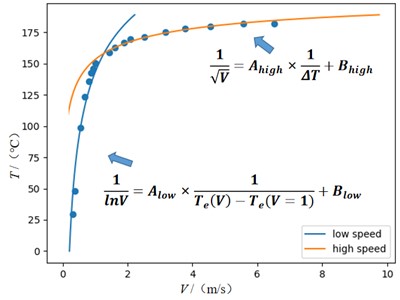
The constant parameters associated with the instrument are simplified to obtain the relationship between $V$ and $T$ satisfied at high and low air speeds.

High air speed:

12

\frac{1}{\sqrt{V}} = A_{h i g h} * \frac{1}{Δ T} + B_{h i g h} .

Low air speed:

13

\frac{1}{l n (V)} = A_{l o w} * \frac{1}{T_{e} (V) - T_{e} (V = 1)} + B_{l o w} .

Eqs. (12-13) give the relationship between air speed and temperature at different air speeds.

3. Design scheme

3.1. Design route

The apparatus comprises four integral modules: an air speed field environment module, a standard air speed measurement module, a temperature measurement module, and a circuit measurement module. A variable wind field is generated through a blower, while a standard anemometer is employed to gauge the air speed precisely at the hot wire's location. Infrared thermal imaging is utilized for capturing the temperature of the hot wire. The circuit is intricately engineered to convert variations in resistance, stemming from temperature fluctuations in the hot wire, into corresponding alterations in circuit current. This facilitates the establishment of a relationship between current and air speed. The design systematically addresses instrumental system errors and the microamp file sensitivity of the digital multimeter, ensuring the selection of optimal parameters for the associated instruments. Fig. 1 illustrates the nuanced design concepts in detail.

The hot wire is intricately integrated into the circuit, arranged in parallel with a resistor box. A digital multimeter, along with an adjustable voltage source, is serially connected to the resistor box branch, and the entire circuit is powered by a current source. Measurement of the current within the resistor box is facilitated by the microampere scale of the digital multimeter, thereby enabling the determination of the hot wire’s resistance variations. The circuit configuration is visually depicted in Fig. 2. Eq. (14) succinctly captures the system dynamics derived from the interplay of voltages across the two branches and the circulating current within the circuit:

14

\{\begin{array}{l} I_{r} r = I^{'} (R + R_{A}) + U, \\ I = I_{r} + I^{'} . \end{array}

Fig. 1Experimental design idea diagram

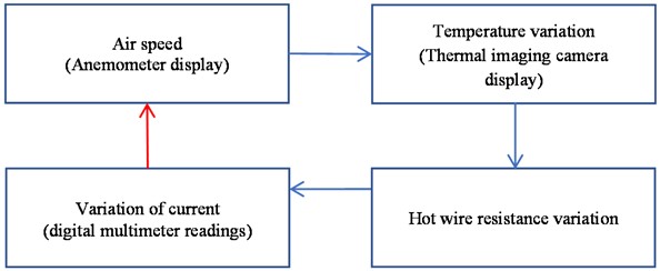
Fig. 2Circuit design diagram

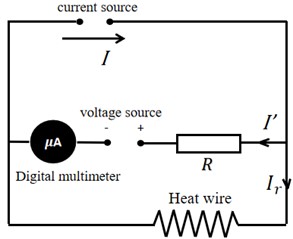
The digital multimeter’s microamp setting reads:

15

I^{'} = \frac{I r - U}{R + R_{A} + r},

where $I$ is the current of the current source; $I^{'}$ is the current of the digital multimeter; $I_{r}$ is the current flowing through the hot wire; $r$ is the resistance of the hot wire; $R$ is the resistance value of the resistance box; $R_{A}$ is the internal resistance of the digital multimeter; $U$ is the voltage of the voltage source.

Adjust the voltage source so that when there is no wind the digital multimeter microamp gear indicates 0. Then there is $r = U / I$ . Assume that when there is a wind field, the electric heating wire resistance changes to $Δ r$ , the digital multimeter microamp gear indicates the following:

16

Δ I = \frac{I Δ r}{R + R_{A} + r} .

Therefore, the variation of the resistance of the hot wire can be obtained as:

17

Δ r = \frac{(R_{A} + R + \frac{U}{I}) Δ I}{I - Δ I} .

Upon scrutiny of Eq. (16), it becomes evident that the resistance value, denoted as $R$ in this circuit, significantly influences the measurement sensitivity of the system. A diminutive $R$ amplifies the sensitivity, making the circuit more responsive to unit changes in current-induced resistance alterations, albeit at the cost of heightened measurement uncertainty. Conversely, a larger $R$ diminishes circuit uncertainty, albeit at the expense of reduced sensitivity. Consequently, a meticulous analysis of uncertainty is imperative to ascertain the optimal $R$ value. The relative uncertainty, articulated in Eq. (17), is derived as follows:

18

\frac{U_{Δ r}}{Δ r} = \sqrt{\sum_{i = U, I, Δ I, R + R_{A}} {(\frac{\partial l n Δ r}{\partial i} U_{i})}^{2}} .

The uncertainties of the relevant instruments are known from the sensitivity of the instruments as follows: $U_{R + R_{A}} =$ 0.1 Ω, $U_{I} =$ 0.001 A, $U_{U} =$ 0.01 V, $U_{Δ I} =$ 0.1 μA.

After bringing them into Eq. (18), we get:

19

U_{Δ r} = \sqrt{2 {(\frac{1}{1000})}^{2} + {(\frac{1}{10 R})}^{2}} .

The sensitivity of hot wire resistance measurement can be obtained from Eq. (17):

20

S_{Δ r} = \frac{d Δ r}{d Δ I} = \frac{I (R_{A} + R) + U}{(I - Δ I)^{2}} .

Considering that the resolution of the multimeter is 0.1 μA; it is necessary to control $∆ I$ in the range of 0-500 μA. Therefore, the measurement sensitivity is $S_{Δ r} \approx R \times 1 \times 1 0^{- 7}$ . When the sensitivity and uncertainty are equal, $R \approx$ 10⁴Ω; the measurement sensitivity of the resistance is obtained as 10^-3Ω. When gradually increasing the air speed, there is an extremely obvious change in the current expression. Therefore, it shows that the circuit and the experimental setup can be used to measure the air speed.

3.2. Apparatus and materials

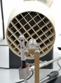
The experimental apparatus, illustrated in Fig. 3, encompasses the utilization of specific instruments and materials. A blower with adjustable air speed (LEYBOLD DIDACTIC GMBH, 37304) serves as the air speed field environment module. The standard air speed measurement module incorporates a SMART SENSOR anemometer (ST866A) strategically positioned near the hot wire, as depicted in Fig. 4.

Fig. 3The assembled hot wire anemometer apparatus

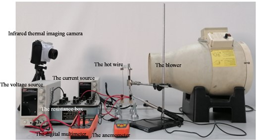
For temperature measurement, an infrared thermal imaging camera (FOTRIC, 224s) is employed to capture comprehensive temperature changes in the hot wire. The circuit measurement module is comprised of essential components: two power supplies (UNI-T,3315TFL-II) functioning as a constant current source to ensure circuit stability and a constant voltage source for adjusting reverse voltage, a VICTOR digital multimeter (VC9805A) for measuring weak current, and a resistor box with adjustable resistance based on design accuracy. Furthermore, the resistor box allows precise adjustment of resistance values in accordance with the experimental design. The hot wire, formed by winding a 0.200 mm diameter iron wire into a spiral shape with dimensions of 8.00 mm in diameter and 35.00 mm in length, is affixed to a bracket, as shown in Fig. 5. The experimental conditions maintain a temperature of 25.0 °C and humidity ranging between 58 % to 63 %.

Fig. 4Structure and fixing method of hot wire

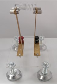
Fig. 5Location of the hot wire and anemometer in the wind field

4. Results and discussion

4.1. Relationship between current and temperature

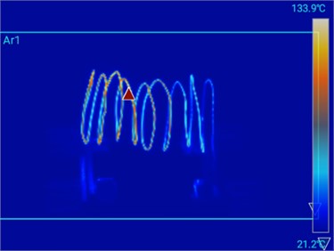
The thermal characteristics of the hot wire were documented through infrared thermography, and the corresponding temperatures were systematically recorded. Fig. 6 illustrates the thermal profile of the hot wire captured by the infrared thermal imaging camera. Concurrently, the current flowing through the circuit was meticulously recorded using the current mode of the digital multimeter. Subsequently, a temperature-current graph was generated, depicted in Fig. 7, wherein different air speed conditions were considered.

Fig. 6Schematic diagram of the hot wire temperature recorded by the thermal imaging camera

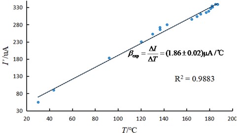
The current was subjected to a linear fit against temperature to ascertain its slope $β_{e x p} = \frac{Δ I}{Δ T} =$ (1.86±0.02) μA/K. Theoretical value $β_{t h e} = \frac{Δ I}{Δ T} = \frac{1 0^{- 6} (R_{A} + R + \frac{U}{I})}{(I - Δ I) α R_{e} (0)} =$ 1.84 μA/K, as per Eq. (7) and (17), were compared with experimental results, revealing a notable consistency between the two. The observed linear relationship between current and temperature, coupled with the convergence of theoretical and experimental outcomes within the margin of error, underscores the viability of employing current as a means to characterize temperature. This concurrence supports the exploration of the experimental relationship between air speed and temperature through current analysis.

Fig. 7Relationship curve between current and temperature at different air speeds

4.2. Relationship between the air speed and hot wire temperature

The air speed in proximity to the hot wire was quantified using an anemometer, while the temperature of the hot wire was systematically documented employing a thermal imaging camera. Concurrently, the current coursing through the constant-value resistor box was precisely registered using a digital multimeter within the microampere range. The datasets of current and temperature, acquired under various air speed conditions, are graphically depicted in Fig. 8.

Fig. 8Relationship between current and temperature at different air speeds

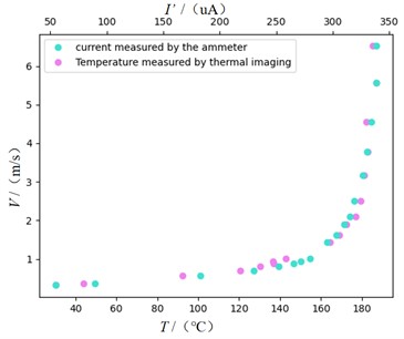
According to the Eqs. (12-13) the digital multimeter microamp gear indication and the thermal wire temperature taken by the infrared camera were fitted in two different intervals of low and high air speed, as shown in Fig. 9. The correlation coefficients and expressions can be obtained as follows.

High air speed: $\frac{1}{\sqrt{V}} = \frac{550}{Δ T} - 2.6$ ; $R^{2} = 0.975$ .

Low air speed: $\frac{1}{l n (V)} = \frac{66.1}{T_{e} (V) - T_{e} (V = 1)} - 0.18$ ; $R^{2} = 0.991$ .

From the correlation coefficient $R^{2}$ it can be seen that the data fitting results are in general agreement with the theoretical formula. Therefore, the hot wire anemometer can be designed for different air speed intervals according to this formula.

Fig. 9Fitting curve of air speed with temperature

4.3. Anemometer sensitivity analysis

From the previous analysis of the sensitivity of resistance measurement, it is clear that the minimum division of temperature is: $S_{T} = \frac{Δ r_{m i n}}{α \frac{U}{I}} \approx$ 5×10^-2 K.

When the air speed is in the range of 0-1.00 m/s, the measurement sensitivity is $Δ V_{m i n} = (\frac{d U}{d I}) * β * S_{T} \approx$ 0.001 m/s.

When the air speed is greater than 1.00 m/s:

21

Δ V_{m i n} = {(\frac{d U}{d I})}_{V > 1 m / s} * β * S_{T} = \frac{2 A_{h i g h} * \frac{1}{Δ I^{2}} * β * S_{T}}{(A_{h i g h} * \frac{1}{Δ I} + B_{h i g h})^{3}} .

The relationship between air speed measurement sensitivity and the air speed range is delineated by Eq. (21). Notably, a simple anemometer exhibits variable sensitivity across distinct air speed intervals, with sensitivity diminishing as air speed increases. Consequently, the worst sensitivity within each interval serves as the basis for establishing three discrete measurement sensitivities across the air speed spectrum. The ensuing outcomes are presented in Table 1.

Table 1Measurement sensitivity of different ranges of anemometer

Measurement sensitivity (m/s)	Air speed measuring range (m/s)
0.001	< 1.000
0.01	1.00-3.00
0.1	3.0-16.0

5. Conclusions

Grounded in the foundational principles of thermal equilibrium, our research embarked on a comprehensive investigation into the intricate relationship between hot wire temperature and air speed. Our methodical approach encompassed the creation of a variable air speed field, the meticulous construction of a bespoke hot wire, the design of an innovative measurement circuit, and the seamless integration of these components into an advanced air speed meter. To probe the correlation between current and temperature, we leveraged both a standard anemometer and an infrared thermal imager, employing these tools to scrutinize the dynamic interplay between air speed and the resultant thermal effects on our custom hot wire. The acquired data was subjected to rigorous analysis, allowing us to not only establish but also validate the anticipated relationship between air speed and current across diverse ranges. Remarkably, the experimental results consistently mirrored the predictions derived from theoretical considerations, affirming the robustness and reliability of our developed air speed meter. One noteworthy aspect of the investigation was the meticulous calculation of measurement sensitivity across various air speed ranges. This involved a nuanced consideration of the smallest scale of selected instruments and the inherent uncertainty associated with theoretical formulas. The air speed meter demonstrated exceptional measurement sensitivity, emerging as a dependable instrument capable of furnishing precise data across a spectrum of air speed conditions. Moreover, the study shed light on the linear relationship between temperature and current in the microampere meter, unveiling the potential utility of electric current as a means for accurate temperature measurements in similar experimental setups. This finding not only enhances the versatility of our air speed meter but also opens avenues for further exploration into leveraging electric current for nuanced temperature assessments.

In summation, our research yields compelling evidence regarding the effectiveness and reliability of the developed air speed meter. Beyond serving as a testament to the meticulousness of our methodology, the study contributes invaluable insights into air speed measurement methodologies, setting the stage for continued exploration into the multifaceted applications of electric current in the realm of precise temperature measurements. This innovative approach not only advances the field of fluid dynamics but also holds promise for diverse scientific and industrial applications where accurate air speed measurement is of paramount importance.

References

P. Ligęza, “Method of testing fast-changing and pulsating flows by means of a hot-wire anemometer with simultaneous measurement of voltage and current of the sensor,” Measurement, Vol. 187, p. 110291, Jan. 2022, https://doi.org/10.1016/j.measurement.2021.110291

Publisher
Paweł Ligęza and Paweł Jamróz, “A hot-wire anemometer with automatically adjusted dynamic properties for wind energy spectrum analysis,” Energies, Vol. 15, No. 13, pp. 1–11, 2022.

Publisher
M. Güçyetmez, S. Keser, and E. Hayber, “Wind speed measurement with a low-cost polymer optical fiber anemometer based on Fresnel reflection,” Sensors and Actuators A: Physical, Vol. 339, p. 113509, Jun. 2022, https://doi.org/10.1016/j.sna.2022.113509

Publisher
G. Canut et al., “Turbulence fluxes and variances measured with a sonic anemometer mounted on a tethered balloon,” Atmospheric Measurement Techniques, Vol. 9, No. 9, pp. 4375–4386, Sep. 2016, https://doi.org/10.5194/amt-9-4375-2016

Publisher
G. Liu, W. Hou, W. Qiao, and M. Han, “Fast-response fiber-optic anemometer with temperature self-compensation,” Optics Express, Vol. 23, No. 10, pp. 13562–13570, May 2015, https://doi.org/10.1364/oe.23.013562

Publisher
D. A. Johnson and W. C. Rose, “Laser velocimeter and hot-wire anemometer comparison in a supersonic boundary layer,” AIAA Journal, Vol. 13, No. 4, pp. 512–515, Apr. 1975, https://doi.org/10.2514/3.49739

Publisher
W. Thielicke, W. Hübert, U. Müller, M. Eggert, and P. Wilhelm, “Towards accurate and practical drone-based wind measurements with an ultrasonic anemometer,” Atmospheric Measurement Techniques, Vol. 14, No. 2, pp. 1303–1318, Feb. 2021, https://doi.org/10.5194/amt-14-1303-2021

Publisher
R. J. Adamec and D. V. Thiel, “Self heated thermo-resistive element hot wire anemometer,” IEEE Sensors Journal, Vol. 10, No. 4, pp. 847–848, Apr. 2010, https://doi.org/10.1109/jsen.2009.2035518

Publisher
L. Kovasznay and Leslie S. G., “The hot-wire anemometer in supersonic flow,” Journal of the Aeronautical Sciences, Vol. 17, No. 9, pp. 565–572, Sep. 1950, https://doi.org/10.2514/8.1725

Publisher
Andreas Fischer, “Hot wire anemometer turbulence measurements in the wind tunnel of LM wind power,” Technical Report, Wind Energy Department, Technical University of Denmark, 2012.

Search CrossRef
C. Doolan, F. Coton, and R. Galbraith, “Measurement of three-dimensional vortices using a hot wire anemometer,” in 30th Fluid Dynamics Conference, Jun. 1999, https://doi.org/10.2514/6.1999-3810

Publisher
Jie Zhang et al., “Effect on measurements of anemometers due to a passing high-speed train,” Wind and Structures, Vol. 20, No. 4, p. 549, 2015.

Publisher
D. Durì, C. Baudet, J.-P. Moro, P.-E. Roche, and P. Diribarne, “Hot-wire anemometry for superfluid turbulent coflows,” Review of Scientific Instruments, Vol. 86, No. 2, pp. 167–231, Feb. 2015, https://doi.org/10.1063/1.4913530

Publisher
N. I. Mikheev, A. V. Sakhovsky, K. R. Khairnasov, and D. V. Kratirov, “Heat-transfer regularities of the anemometric wire,” Thermophysics and Aeromechanics, Vol. 17, No. 2, pp. 173–180, Nov. 2010, https://doi.org/10.1134/s0869864310020022

Publisher
J. Kielbasa, “The hot-wire anemometer/anemometr z grzanym włóknem,” Archives of Mining Sciences, Vol. 59, No. 2, pp. 467–475, 2014.

Publisher
P. Ligeza, “Modeling of complex hot-wire measuring system,” in Optoelectronic and Electronic Sensors IV, Vol. 4516, No. 1, pp. 131–138, Aug. 2001, https://doi.org/10.1117/12.435913

Publisher
J. Coffaro, M. Richardson, R. Bernath, and R. Crabbs, “Sonic anemometer data processing for comparison to optical turbulence theory and simulation,” Journal of the Optical Society of America A, Vol. 39, No. 4, pp. 643–654, Apr. 2022, https://doi.org/10.1364/josaa.441020

Publisher
L. V. King, “On the convection of heat from small cylinders in a stream of fluid: Determination of the convection constants of small platinum wires, with applications to hot-wire anemometry,” Proceedings of the Royal Society of London. Series A, Containing Papers of a Mathematical and Physical Character, Vol. 90, No. 622, pp. 563–570, Sep. 1914, https://doi.org/10.1098/rspa.1914.0089

Publisher
H. Lundström, “Investigation of heat transfer from thin wires in air and a new method for temperature correction of hot-wire anemometers,” Experimental Thermal and Fluid Science, Vol. 128, p. 110403, Oct. 2021, https://doi.org/10.1016/j.expthermflusci.2021.110403

Publisher
E. Özahi, M. Çarpınlıoǧlu, and M. Y. Gündoǧdu, “Simple methods for low speed calibration of hot-wire anemometers,” Flow Measurement and Instrumentation, Vol. 21, No. 2, pp. 166–170, Jun. 2010, https://doi.org/10.1016/j.flowmeasinst.2010.02.004

Publisher
H. Kaplan, Practical Applications of Infrared Thermal Sensing and Imaging Equipment, Third Edition. SPIE, 2007, https://doi.org/10.1117/3.725072

Publisher
P. C. Jena, “Design and analysis of heat exchanger by using computational fluid dynamics,” in Sustainable Engineering Products and Manufacturing Technologies, Elsevier, 2019, pp. 159–176, https://doi.org/10.1016/b978-0-12-816564-5.00006-2

Publisher

About this article

Received

15 September 2023

Accepted

28 December 2023

Published

03 January 2024

DOI

https://doi.org/10.21595/jme.2023.23637

Keywords

hot wire

anemometer

uncertainty

sensitivity

Acknowledgements

This project is funded Experimental Technology Research Project of Zhejiang University in 2022 (SYBJS202205).

Data Availability

The datasets generated during and/or analyzed during the current study are available from the corresponding author on reasonable request.

Author Contributions

Xingxing Yao: funding acquisition, investigation, resources, validation, writing-review and editing, writing-review and editing. Fanhao Shen: conceptualization, data curation, formal analysis. Yuan Zheng: resources, writing-review and editing. Ting Xiao: investigation, writing-review and editing.

Conflict of interest

The authors declare that they have no conflict of interest.

This is an open access article distributed under the Creative Commons Attribution License, which permits unrestricted use, distribution, and reproduction in any medium, provided the original work is properly cited.

Previous article in issue Previous Next article in issue Next

Research article

2022 08 25

Design and accuracy test of polar moment of inertia measuring equipment for projectile and rocket

Liwei Sun, Shukun Wang, Haokun Wang, Weihong Zhao, Junye Li, Chunmin Shang

Research article

2022 06 30

Reliability of quantitative risk models: a case study from offshore gas production platform

Mohamed Attia, Jyoti Sinha

Research article

2021 11 05

Temperature difference measurement with using two RTD sensors as example of evaluating uncertainty of a vector output quantity

Adam Idzkowski, Zygmunt Warsza

Research article

2021 05 24

Development of a MEMS hotplate-based photoacoustic CO2 sensor

Lucky A. Ishaku, David Hutson, Des Gibson

X. Yao, F. Shen, Y. Zheng, and T. Xiao, “An assembled hot wire anemometer design,” Journal of Measurements in Engineering, Vol. 12, No. 1, pp. 138–148, Jan. 2024, https://doi.org/10.21595/jme.2023.23637

Copy Extrica

Copied to clipboard!

TY  - JOUR
DO  - 10.21595/jme.2023.23637
UR  - https://doi.org/10.21595/jme.2023.23637
TI  - An assembled hot wire anemometer design
T2  - Journal of Measurements in Engineering
AU  - Yao, Xingxing
AU  - Shen, Fanhao
AU  - Zheng, Yuan
AU  - Xiao, Ting
PY  - 2024
DA  - 2024/01/03
PB  - Extrica
SP  - 138-148
VL  - 12
IS  - 1
SN  - 2335-2124
SN  - 2424-4635
ER  - 

Copy Ris

Copied to clipboard!

 @article{Yao_2024, title={An assembled hot wire anemometer design}, volume={12}, ISSN={2424-4635}, url={https://doi.org/10.21595/jme.2023.23637}, DOI={10.21595/jme.2023.23637}, number={1}, journal={Journal of Measurements in Engineering}, publisher={JVE International Ltd.}, author={Yao, Xingxing and Shen, Fanhao and Zheng, Yuan and Xiao, Ting}, year={2024}, month=jan, pages={138–148} }

Copy Bibtex

Copied to clipboard!

[1]X. Yao, F. Shen, Y. Zheng, and T. Xiao, “An assembled hot wire anemometer design,” Journal of Measurements in Engineering, vol. 12, no. 1, pp. 138–148, Jan. 2024, doi: 10.21595/jme.2023.23637.

Copy IEEE

Copied to clipboard!

Yao, Xingxing, Fanhao Shen, Yuan Zheng, and Ting Xiao. “An Assembled Hot Wire Anemometer Design.” Journal of Measurements in Engineering 12, no. 1 (January 3, 2024): 138–48. https://doi.org/10.21595/jme.2023.23637.

Copy Chicago

Copied to clipboard!

An assembled hot wire anemometer design

Abstract

1. Introduction

2. Theoretical basis

3. Design scheme

3.1. Design route

3.2. Apparatus and materials

4. Results and discussion

4.1. Relationship between current and temperature

4.2. Relationship between the air speed and hot wire temperature

4.3. Anemometer sensitivity analysis

5. Conclusions

References

About this article

Related Articles