Abstract
The vehicle-mounted tanks face prominent challenges in balancing dynamic safety, including vibration resistance and fatigue durability under complex transportation conditions. A rigid-flexible coupled finite element model, consisting of the base, tank body, and frame, was established. Vibration response analysis was conducted in accordance with ride comfort standards and road excitation requirements. Rigid-flexible coupled simulations were implemented with consideration of vertical acceleration inputs and road unevenness. For random vibration, power spectral density analysis demonstrated that the tank structure was prone to resonance in specific frequency bands. For structural optimization, key dimensions were selected as design variables, including vertical thickness, longitudinal thickness, middle width, and lateral width. An optimization mathematical model was established, and the Sequential Quadratic Programming (SQP) algorithm was adopted to solve the constrained nonlinear multi-objective optimization model. Through optimization calculations, the structure achieved 4.93 % reduction in mass, 37.3 % decrease in stress, and 37.1 % increase in the first-order natural frequency, thereby effectively balancing the requirements of lightweight design, structural strength safety, and anti-resonance performance. This study provided a comprehensive methodology for the dynamic analysis and optimization of vehicle-mounted tank containers, offered key technical support for advancing innovative studies in transportation and vibration engineering.
Highlights
- A rigid-flexible coupled finite element model, consisting of the base, tank body, and frame, was established.
- Rigid-flexible coupled simulations were implemented with consideration of vertical acceleration inputs and road unevenness.
- For random vibration, power spectral density analysis demonstrated that the tank structure was prone to resonance in specific frequency bands.
1. Introduction
In the modern transportation sector, the safety and reliability have become the core indicators for evaluating their performance. As a key component for storing fuel, the dynamic mechanical behavior of the vehicle-mounted tank directly affects the overall safety and service life of the transportation mission. With the rapid development of the automotive industry, the driving conditions that needs to be taken into account in the design have become increasingly complex, ranging from frequent starts and stops on urban roads to continuous high-speed driving on highways, and even to bumpy and shock-prone off-road environments. The vehicle-mounted tank is constantly subjected to multi-source coupled loads such as engine vibration, road excitation, and alternating load. These dynamic loads can cause vibration responses in the vehicle-mounted tank structure, and long-term exposure may lead to weld cracking, structural fatigue failure, and even serious safety accidents such as fuel or gas leakage. According to relevant data statistics, about 15 % of mechanical failures in vehicle faults are related to vibration fatigue. Therefore, in-depth research on the vibration response characteristics of the tank has significant practical engineering significance.
With the development of computer technology and numerical simulation methods, the finite element method has become the mainstream tool for structural dynamics analysis due to its ability to discretize complex structures and its high-precision calculation advantages. Through finite element models, the vibration modes, stress distribution, fatigue life and other characteristics of the structure under different excitation conditions can be quantitatively analyzed. Representative studies include Yamashita [6] proposed an analysis method for vibration energy propagation in rigid-flexible coupling systems, evaluating and optimizing vibration control strategies through modal energy flow. Marano [7] designed exoskeleton structures based on stochastic multi-objective optimization methods to enhance the seismic performance of buildings, balancing safety and economy. Talebitooti [8] proposed a modal algorithm that terminates the series by selecting a sufficient number of modes. Therefore, convergence checks were carried out in three-dimensional structures for different frequencies and shell sizes, which can determine the appropriate number of modes required for dynamic analysis. Flores [9] employed the NSGA-III algorithm to optimize the vehicle suspension system, balancing ride comfort and handling stability. Lankarani [10] established a contact and collision model of a rigid-flexible coupling system with a clearance hinge and analyzed the vibration transmission characteristics. Ambrosio [10] optimized the damping parameters for the rotor-bearing system to reduce the vibration response and enhance stability. Greco [11] studied the fluid-structure interaction vibration characteristics of composite material liquid storage tanks and proposed structural optimization schemes. Bestle [12] established a rigid-flexible coupling model of tracked vehicles with clearance hinges and analyzed the vibration characteristics during operation.
With the advancement of vehicle transportation engineering, the structural configurations of tank containers mounted on vehicles have become increasingly diverse, leading to more complex vibration response characteristics [13, 14]. By employing multi-condition simulation and multi-objective optimization techniques, an efficient analytical approach can be established for the research and development phase. This approach not only effectively bridges the gap between theoretical research and engineering practice, but also serves as a critical foundation for enhancing overall vehicle safety and driving technological innovation within the automotive industry. In order to ensure that the tank container can meet the working requirements under different excitation vibrations, and to improve the rationality of the structural design and reduce the mass redundancy, the dynamic response is studied in this paper by combining the simulation method and the analytical method. Compared to previous studies, the innovation of the research mainly lies in three aspects: (1) A layered rigid-flexible coupling modeling strategy was proposed. The bogie was modeled as a rigid body, and the tank was modeled as a flexible body. Through this approach, a dynamic closed loop between the bogie and the tank was constructed, and the stiffness difference between the bogie and the tank in engineering practice was matched. (2) A vibration correlation model covering the global and local scales was established. The deformation characteristics of each order of mode and the risk frequency bands were clarified, and the accurate mapping of resonance frequency bands and weak positions was realized. This provided a targeted basis for risk prediction such as weld fatigue and local displacement fluctuation. (3) A multi-objective optimization process consisting of variable screening, response surface modeling, and SQP (Sequential Quadratic Programming) solution was constructed. The influence of design variables on the objectives was quantified by correlation coefficients. A high-precision response surface model was used to replace the finite element simulation, and the directional improvement of performance was achieved.
2. Analysis of dynamic characteristics
2.1. Theoretical analysis of road vibration
Road vibration analysis of vehicle-mounted tank requires modal calculation first. Modal analysis can simplify complex structures into corresponding modal shapes, and then perform dynamic response calculations based on these modal shapes, thus greatly simplifying mathematical calculations. Therefore, the key to conducting modal analysis on a system lies in extracting the system’s eigenvectors. The eigenvalues are the natural frequencies of the structure, and calculating them is beneficial for avoiding potential system resonance during the design phase. For a linear time-invariant system with degrees of freedom, in common dynamic problems, its dynamic equilibrium equation is as follows:
where is the mass matrix, is the system stiffness matrix and is the displacement response of each point in the system.
Under the condition of undamped free vibration, Eq. (1) can also be expressed as:
where is the mode shape vector, and is the natural angular frequency.
The actual excitation vibration during road travel cannot be described by a deterministic function. It is necessary to analyze it using the statistical characteristics of a random process, such as power spectral density. The core is to solve the response statistics of the structure under random excitation. Power spectral density (PSD) can describe the distribution of response energy in the frequency domain and is a core input and output parameter in random vibration analysis. It can be expressed using the Fourier transform relationship as:
where is the auto-correlation function.
For modal decoupling, it needs to be decomposed into independent SDOF systems. The th order modal force can be expressed as:
where represents the foundation vibration transmitted from the road surface vibration.
2.2. Establishment of the rigid-flexible coupling model
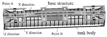
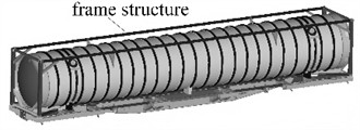
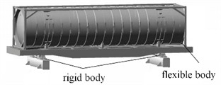
Since vehicle-mounted tank is specially designed for transporting liquids, gases and powdered goods, they have distinctive structural features. As shown in Fig. 1(a) and Fig. 1(b), vehicle-mounted tank system mainly consists of a base, a tank body and a frame. The tank body is mostly cylindrical. The external frame structure conforms to international standard sizes such as 20 feet and 40 feet, is made of high-strength steel, and is equipped with corner fittings for easy loading and unloading, which also has the functions of bearing weight and protecting the tank body. To better achieve vibration response analysis, the rigid-flexible coupling technology is applied. To ensure the reliability of the dynamic characteristic analysis model, the bogie is set as a rigid body and the tank as a flexible body. The rigid-flexible coupling characteristics of the on-board system present a more explicit hierarchical relationship. As the rigid base for load-bearing and force transmission, the movement of the bogie directly determines the base excitation state of the tank, while the flexible deformation of the tank reacts back to the bogie through the coupling interface, forming a dynamic closed loop, as shown in Fig. 1(c). This setting is more in line with the engineering reality where the structural stiffness of the bogie is much higher than that of the tank.
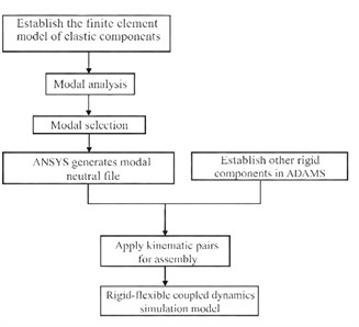
The rigid-flexible coupling dynamics modeling process based on ANSYS and ADAMS is shown in Fig. 1(d). Rigid-flexible coupling analysis necessitates the creation of a Modal Neutral File (MNF), which integrates multibody dynamics with finite element analysis [15, 16]. The process begins with establishing a finite element model of the flexible body, followed by mesh division as illustrated in Fig. 2 and material property definition as detailed in Table 1. Through modal analysis, relevant modal data – including natural frequencies, mode shapes, and mass matrices – can be extracted for the required modal orders. The modal neutral file is then generated via the interface. During this procedure, it is essential to verify the integrity of the modal data, ensure the consistency of rigid-flexible coupling interface parameters, and confirm that the final file is compatible with the dynamic simulation solver to facilitate subsequent dynamic characteristic analysis of the rigid-flexible coupling system. To balance computational accuracy and efficiency, it is necessary to screen out the modes that have a significant impact on the dynamic response and ignore the higher-order secondary modes.
Fig. 1The structure composition and modeling process of vehicle-mounted tank
a) The view at the bottom of the model
b) The view at the front of the model
c) The definitions of rigid and flexible bodies
d) The process of rigid-flexible coupling modeling
Fig. 2Results of mesh division
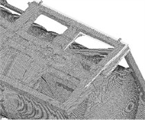
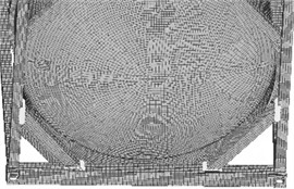
Table 1Results of mesh division
Component | Common material | Elastic modulus (GPa) | Poisson’s ratio | Density (kg/m³) | Yield strength (MPa) |
Base | Low carbon steel (Q235) | 205 | 0.29 | 7850 | 235 |
Tank Body | Stainless steel (304) | 193 | 0.30 | 7930 | 205 |
Frame | High-strength low-alloy steel (Q355) | 210 | 0.28 | 7800 | 355 |
2.3. Analysis of modal characteristics
The analysis results of the first four – order modal shapes of the tank container are presented in Fig. 3. It can be observed that the first – order mode exhibits a bending vibration pattern along the length direction. The relative displacement at both ends of the tank container is relatively small, while the bending deformation in the middle region is rather significant. The tank body, base and frame jointly present this kind of vibration mode with the long axis bending. The second - order modal shape is more intricate. Apart from retaining a certain long - axis bending tendency, relatively distinct local vibration responses emerge at the connection parts between the tank body and the frame as well as some areas of the base. The overall vibration distribution is no longer a simple uniform bending along the long axis; instead, a vibration form with a stronger hierarchical sense is formed between the local and the overall. The third - order modal shape shows more local vibration characteristics. The variation in vibration displacement of the tank body itself and the surrounding support frame structure is more prominent, and relatively obvious vibration differences occur in local regions (such as different segments of the tank body and certain crossbeams of the frame). The fourth - order mode vibration is mainly concentrated in specific regions. For some local structures of the tank container, like the intermediate connection structure of the base, the difference in vibration displacement amplitude is substantial, presenting a localized vibration mode, and there is no obvious long - axis or overall coordinated vibration trend on the whole.
Fig. 3The first four modal shapes
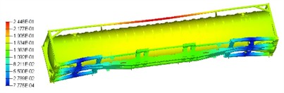
a) The first modal shape (7.26 Hz)
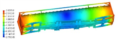
b) The second modal shape (9.33 Hz)
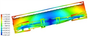
c) The third modal shape (12.25 Hz)
d) The fourth modal shape (13.77 Hz)
2.4. Vibration response analysis based on ride comfort standards
In the ride comfort analysis of ADAMS, it is necessary to specify the vibration input (road unevenness) and vibration response quantities. According to road standards, the C-class road unevenness coefficient is set to 256e-6 m3, the vertical acceleration is 0.315 m/s2, the relative dynamic load is 0.95, and the dynamic deflection is 8 mm. To achieve the shock absorption effect of tank containers, vibration isolation elements are arranged between the rigid and flexible models, and the stiffness and damping curves of their connections are shown in Fig.4.
Fig. 4The definition of contact with coupling of rigidity and flexibility
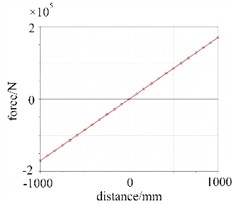
a) Contact stiffness curve
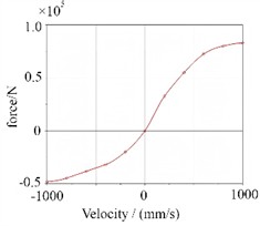
b) Contact damping curve
When a vehicle travels on a road with undulations or unevenness, the displacement excitation from the road surface will be transmitted to the rigid – flexible coupled structure of the tank container through systems such as the suspension. The stiffness curve reflects the structure’s ability to resist such displacement deformation. The linear stiffness characteristic means that the deformation of the structure within the elastic range has a linear relationship with the applied load. Through this curve, the magnitude of the force generated inside the structure under different road surface displacement inputs can be quantitatively analyzed, and then the static and dynamic deformation degrees of the structure caused by road surface unevenness can be evaluated. This is crucial for determining whether structures such as tank containers will affect the safety and stability of themselves and the internal goods due to excessive deformation during driving. The main role of damping in road ride comfort is to consume vibration energy and attenuate vibration responses. When a vehicle is driving on the road, due to the unevenness of the road surface, the rigid – flexible coupled structure will vibrate, and the change in vibration speed will cause a change in damping force. It can be seen from the curve that as the vibration speed increases, the damping force first rises rapidly and then the growth slows down. This indicates that when the vibration speed is low, the damping can quickly provide a large force to attenuate the vibration; when the speed reaches a certain level, the growth of the damping force tends to be stable, and it can still continue to play a role in attenuating the vibration. Using this damping curve, the magnitude of the damping force at different vibration speeds can be accurately calculated, thereby analyzing the dissipation of vibration energy, evaluating the vibration attenuation efficiency of the rigid – flexible coupled system under road excitation, and then determining the ride comfort of the vehicle when driving, that is, the intensity of vibration felt by passengers or goods. A system with good damping characteristics (which can effectively attenuate vibration) has better road ride comfort.
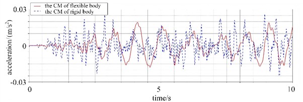
After model coupling, the variation law of the centroid acceleration of the rigid body and the flexible body with time is presented in Fig. 5, which can reflect the frequency characteristics of their acceleration changes. From the frequency perspective, the fluctuation frequency of the centroid acceleration of the flexible body is relatively higher. Specifically, within the same time interval, the number of fluctuations of its acceleration curve is greater, implying that the flexible body possesses richer frequency components in the coupled system and is more prone to generating high-frequency acceleration variations. In contrast, the fluctuation frequency of the centroid acceleration of the rigid body is relatively lower, with fewer fluctuation occurrences, indicating that the vibration frequency of the rigid body is relatively low and dominated by low-frequency acceleration changes. Overall, the fluctuation amplitude of the centroid acceleration of the flexible body is relatively larger, with the peak value closer to 0.03 m/s2 and the valley value also closer to –0.03 m/s2. This complies with the requirements of the ISO 2631-1 vibration assessment standard (0.63m/s2). The centroid acceleration of the rigid body fluctuates relatively gently, and its acceleration value lies within the fluctuation range of the centroid acceleration of the flexible body for most of the time. Furthermore, there exists a certain degree of synchronization in the acceleration variation trends of the two. The occurrence moments of fluctuation peaks and valleys are relatively close at multiple time points, yet the specific acceleration values differ, reflecting the distinct acceleration response characteristics of different centroids during motion after the coupling of the rigid body and the flexible body.
Fig. 5The curves of the changes in the center of mass acceleration
To analyze the dynamic mechanical characteristics of the tank container, the load response curves of points A and B shown in Fig. 1(a) were calculated and obtained, as illustrated in Fig. 6. It can be seen that when the vertical impact on the road surface (such as continuous bumps) is transmitted to the edge, the -direction force directly impacts the base, and due to the lack of a symmetrical structure at the edge to counteract the vibration, there are more load peaks. The load amplitude at point B is significantly greater than that at point A because point A is at the edge, and the excitations coming from different directions are relatively difficult to form effective superposition at the edge position. When the vibration is transmitted to the far left, due to the differences in transmission paths and phases, they will weaken each other, thereby reducing the load amplitude. The center position is the convergence point of multiple excitation transmission paths, and excitations from different directions are more likely to superimpose at the center position, resulting in an increase in the total load amplitude.
Fig. 6Dynamic load response
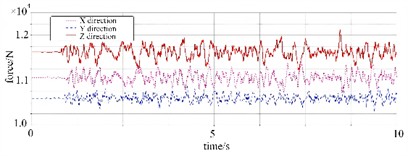
a) Point A
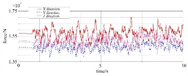
b) Point B
3. Analysis of random vibration under road excitation
3.1. Response of power spectral density
To fit the actual working conditions, road excitation was applied in accordance with the GB4857.23 standard. The power spectral density (PSD) curve, as shown in Fig. 7, serves as a crucial basis for evaluating the reliability of products under transportation vibration conditions. The PSD curve intuitively presents the distribution of vibration energy contained in different frequency components. Under the GB4857.23 standard, the curve below 5 Hz shows a relatively steep trend, indicating that the vibration energy in this frequency band is relatively stable and accounts for a large proportion. This is mainly because low-frequency vibrations usually originate from actions such as slow bumps, acceleration, or deceleration during the vehicle's operation.
Fig. 7PSD power spectrum curve of road excitation
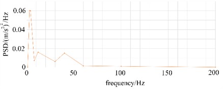
As the frequency increases to the 5-40 Hz range, the PSD curve fluctuates, and its amplitude decreases. This frequency band is related to factors such as vehicle engine vibration, wheel rotation, and common road irregularities. The combined effect of these factors leads to a significant increase in vibration energy within this frequency interval, exerting a substantial impact on transported goods. In the high-frequency band, i.e., above 40 Hz, the amplitude of the PSD curve gradually declines, indicating a gradual reduction in high-frequency vibration energy. High-frequency vibrations are mostly caused by factors such as minor road irregularities and tiny resonances of vehicle components. Although their energy is relatively low, long-term effects may cause fatigue damage to the precision components of the product. The linear slopes of different frequency bands vary, reflecting the different rates at which the vibration energy of different frequency components changes with frequency. Moreover, compared with some other transportation vibration standards, the PSD curve under this standard has a relatively higher amplitude in the mid-frequency band (10-30 Hz). This is because this frequency band concentrates multiple vibration factors that have a significant impact on transported goods, such as the coupling effect between the vehicle suspension system and road excitation.
In the transportation of tank containers, road bumps and vehicle start-stop impacts will all be converted into acceleration excitation. Through the analysis of acceleration response, it can predict to a certain extent whether the structure of the container will be damaged due to vibration overload in a random vibration environment, avoiding the risks of leakage and deformation during transportation. Under the random vibration conditions of the road surface, the acceleration responses at points A and B can be obtained, as shown in Fig. 8. It can be seen that the acceleration curve of point A fluctuates significantly within the range of –10 to 10 m/s² in the direction, showing a wide-frequency and high-frequency oscillation feature, with frequent peaks throughout the entire period. In the direction, the curve fluctuates within –1 to 2 m/s2, mainly characterized by small-amplitude and high-frequency vibrations, with dense peaks and higher amplitudes in the 5-15 second interval. The vibration amplitude of point B in the direction is significantly larger than that of point A, with a greater standard deviation, but it is more stable in the direction.
Fig. 8The acceleration responses of point A and point B
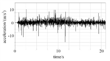
a) Point A in direction
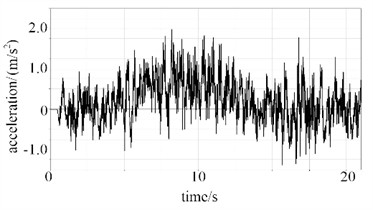
b) Point A in direction
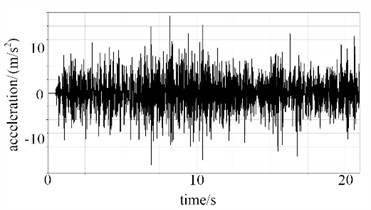
c) Point B in direction
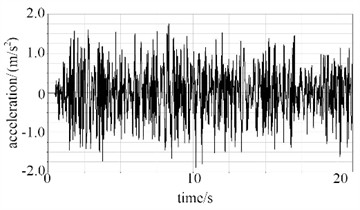
d) Point B in direction
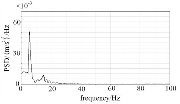
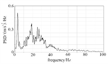
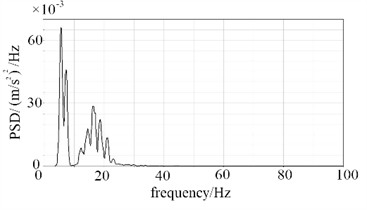
To analyze the vibration response under frequency domain conditions, the acceleration response curve was transformed, and the PSD response result is shown in Fig. 9. For point A, a significant peak observed in the 5-15 Hz range suggests that the structure may experience resonance within this frequency band. At this specific frequency, the PSD value is markedly higher than at other frequencies, indicating that structural components are subjected to greater stress during vibration, thereby increasing the likelihood of fatigue cracks and other strength-related issues. For point B, the dominant peak in the 0-5 Hz range corresponds to the first natural frequency of the overall container frame and tank structure. This frequency band is susceptible to coupling with long-wave road irregularities, potentially triggering global resonance that subjects the structure to cyclic stresses far exceeding design limits, thus representing a high-risk zone for weld cracking and support deformation. The secondary peaks within the 5-40 Hz range reflect local vibration modes associated with frame beams and tank stiffeners. These frequencies are prone to resonate with vibrations from the vehicle suspension system and engine idling, resulting in localized stress concentrations and accelerated fatigue damage accumulation. Vibrational energy above 40 Hz can generally be disregarded, as the structure exhibits strong high-frequency filtering capabilities, rendering such frequencies unlikely to pose a significant threat.
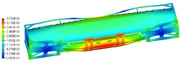
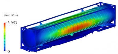
Based on the modal analysis results, the random load is projected onto individual vibration modes to derive the corresponding generalized forces for each mode. According to random vibration theory, the dynamic response of each mode under random excitation is computed using the generalized mass, generalized stiffness, and generalized force of each modal order, in conjunction with the statistical properties of the input random variables. These modal responses are then superimposed to generate the stress distribution contour of the structure under random vibration conditions, as illustrated in Fig. 10. It can be seen that there is stress concentration in the middle of the tank and the area connecting with the base frame, with a peak value of 3.953 MPa. The stress at both ends and the edge of the frame is low and evenly distributed. According to the industry standard (JB/T 4730-2019 Non-destructive Testing for Pressure Vessels), as a pressure-bearing structure, the allowable stress of the tank under vibration should not exceed 80 % of the material's yield strength, which is 164 MPa. According to the results of random vibration analysis, it can be known that the maximum stress of the tank fully meets the safety requirements.
Fig. 9The PSD responses of point A and point B
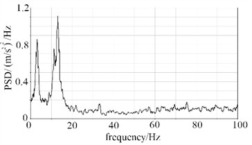
a) Point A in direction
b) Point A in direction
c) Point B in direction
d) Point B in direction
Fig. 10Stress results under random vibration conditions
3.2. Response of fatigue characteristics
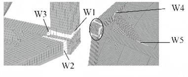
Fatigue life estimation methods under random vibration loads can be broadly categorized into time-domain and frequency-domain approaches. The time-domain method directly analyzes the temporal evolution of structural responses during random vibration, tracking variations in physical parameters such as stress and displacement over time. By integrating cycle counting techniques, this method identifies and quantifies load cycles, which are subsequently used with S-N curve (shown in Fig. 11) and cumulative damage theories, such as Miner’s linear damage rule, to estimate fatigue damage and predict structural life. A key advantage of the time-domain approach lies in its ability to accurately simulate and analyze complex loading histories. However, due to the necessity of processing extensive time-series data, it incurs a relatively high computational cost, often requiring significant computation time and resource allocation. In contrast, the frequency-domain method, which is based on power spectral density, is widely adopted in structural design and durability evaluation for its computational efficiency and consistent results. This method transforms the time-domain response of the structure under random vibration into the frequency domain in the form of PSD. It then analyzes the frequency components, energy distribution, and phase characteristics of the signal using the PSD curve, and combines this information with material S-N curves and fatigue damage accumulation models to estimate fatigue life. As the tank body is an independent standard component that meets the G150 design requirements and has passed the load verification, fatigue analysis is not necessary. Therefore, this paper takes five key welds (shown in Fig. 12) as the research targets to conduct fatigue impact analysis to ensure the overall mechanical performance.
Fig. 11S-N curve
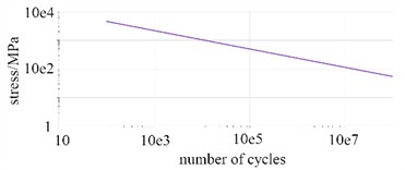
Fig. 12Definition of weld seam
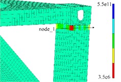
Taking weld seam 1 (W1) as an example, through path setting, the fatigue life and stress variation rules at different nodes can be obtained, as shown in Fig. 13. It can be observed that the majority of node lifespans are concentrated within the range of 1e6 to 1e8 minutes (medium to high fatigue life levels), whereas certain localized nodes (e.g., Node 6 and Node 26) exhibit abrupt reductions in fatigue life. This indicates an uneven distribution of fatigue life, which is closely associated with stress levels and structural features such as openings and welds. The overall stress fluctuates between 0.1 and 0.5 MPa, with Node 1 experiencing the highest stress of 0.45 MPa and Node 14 the lowest stress of 0.15 MPa. Notably, the stress distribution is inversely correlated with the fatigue life distribution, that is, nodes subjected to higher stress exhibit shorter fatigue life, whereas those under lower stress demonstrate longer fatigue life.
Fig. 13Change of fatigue life and stress in weld direction (W1)
a) Cloud map of fatigue life

b) Change of fatigue life

c) Change of stress
The minimum fatigue life and maximum stress of five different welds are shown in Table 2. It can be seen that under random vibration conditions, weld 4 bears the maximum stress, which is 0.488 MPa. This can be taken as the optimization target in the subsequent structural optimization process.
Table 2The minimum fatigue life and maximum stress of different welds
Name of weld seam | W1 | W2 | W3 | W4 | W5 |
Minimum fatigue life / min | 9.65e5 | 1.22e6 | 1.08e6 | 9.04e5 | 9.13e5 |
Maximum stress / MPa | 0.421 | 0.374 | 0.393 | 0.488 | 0.464 |
4. Structural optimization of the base structure
4.1. Design variables and optimization objectives
The base structure serves as a critical component that connects the tank container to the vehicle frame. However, it often suffers from issues such as excessive mass redundancy. Through rational optimization design of the base, the mass and stiffness distributions of the structure can be effectively adjusted. This approach not only enhances the natural frequency to meet specified requirements but also improves the stress distribution, reduces peak stress levels, and ensures a more stable structural response under various dynamic loads, thereby significantly prolonging the fatigue life of the structure [17].
Based on the structural characteristics of the base, the size parameters are defined as design variables, as illustrated in Fig. 14, including vertical thickness (P1), longitudinal thickness (P2), middle width (P3), and lateral width (P4), with their allowable value ranges provided in Table 3. With respect to the optimization objectives, guided by stiffness and strength requirements, the minimum mass (Y1), the minimum stress peak (Y2), and the maximum first natural frequency (Y3) are regarded as the optimization goals. The first natural frequency represents a critical dynamic characteristic of the tank container base. When the external excitation frequency approaches or coincides with this frequency, resonance may occur, resulting in a rapid increase in structural vibration amplitude and a substantial rise in stress levels. This can potentially lead to severe structural damage and safety incidents such as tank leakage. Maintaining a first natural frequency above common external excitation frequencies effectively mitigates resonance risks, thereby ensuring structural integrity and transportation safety of the container.
Fig. 14Definition of design variables for the base structure
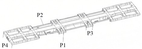
Table 3The range of values for design variables
Name of design variables | P1 | P2 | P3 | P4 |
Initial value / mm | 16 | 12 | 180 | 460 |
Minimum value / mm | 12.8 | 9.6 | 144 | 368 |
Maximum value / mm | 19.2 | 14.4 | 216 | 552 |
4.2. Correlation analysis
In multi-objective optimization, the correlation coefficient between design variables and optimization objectives is a quantitative indicator that measures the degree and direction of the influence of a design variable on a certain optimization objective [18-19]. For instance, for the th design variable and the th objective , the correlation coefficient is defined as:
where is the mean of the th design variable. is the mean of the th objective.
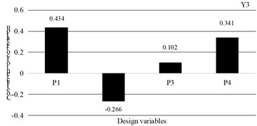
Through calculation, the correlation coefficients between the design variables and the optimization objectives of the base structure of the tank container can be obtained, as shown in Figs. 15-17. It can be seen that the design variables of P1 and P2 have the greatest positive correlation with the mass, which has a crucial impact on weight reduction and can effectively balance mass and stiffness. For the stress peak, the strong negative correlation between P1 and P3 is the greatest. Under the condition of quality being allowed, widening both sides can effectively disperse the load. Although P4 is positively correlated with the stress peak, it can be known through calculation that controlling parameter P4 can avoid local stress concentration. Fine-tuning P2 has a limited effect on reducing stress and can be used as an auxiliary optimization. The correlation between the vertical thickness P1 and the longitudinal thickness P2 with the natural frequency is negative and highly significant. In multi-objective optimization, a trade-off must be carefully balanced among mass reduction, stress control, and frequency improvement. The Pareto optimal solution can be efficiently identified using the sequential quadratic programming algorithm. By integrating physical interpretation with correlation coefficients, the optimization process transitions from blind trial-and-error to precise and informed regulation. This approach provides a clear and systematic path for adjusting design variables in tank container base design, ensuring the achievement of key engineering objectives: minimal mass, stress within allowable limits, and maintained natural frequency.
Fig. 15The correlation coefficient between design variables and Y1

Fig. 16The correlation coefficient between design variables and Y2
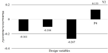
Fig. 17The correlation coefficient between design variables and Y3
4.3. Solution of optimized mathematical model
The performance analysis of tank container usually relies on numerical simulation methods such as finite element analysis, which incurs high computational costs. Response surface function fitting aims to replace complex numerical models with a relatively simple approximate function (response surface function) to quickly predict response values within the design variable space. Based on statistical and mathematical approximation theories, it is assumed that there exists a certain functional relationship between the response and the design variables. By conducting a series of samplings of the design variables and calculating the corresponding response values, these sample data are used to fit a function that can approximately describe their relationship [20].
The error results of each response surface function are shown in Table 4. For the response surface function of mass, the value of the coefficient of determination is 1. This indicates that the response surface model can fully express the variation of mass with design variables, and there is no deviation in the quadratic polynomial relationship between mass and variables, resulting in an extremely high goodness of fit. The root mean square error (RMSE) is extremely small, only 0.00102, which means the average deviation between the mass predicted by the model and the true value from the finite element analysis is negligible, meeting the high-precision requirements of engineering for mass control. Both the relative average absolute error (RAAE) and the relative mean absolute error (RMAE) are 0, demonstrating that the predicted mass values of all sample points are completely consistent with the true values. For the response surface function of the peak stress, the model can explain 97.9 % of the stress variation, and only 2.1 % of the deviation stems from the complex effect of local stress concentration, resulting in an excellent overall goodness of fit. The average deviation of 1.278 MPa is far lower than the allowable stress of the material, and the deviation ratio is only 0.54 %, which is much smaller than the 5 % engineering acceptable threshold and will not affect the judgment of whether the stress exceeds the limit. The mean absolute error of the first-order natural frequency is 2.861 Hz, with an extremely small deviation. This enables accurate prediction of frequency changes under different combinations of design variables, ensuring that the frequency of the optimized base is far from the risk of resonance.
Table 4The result of error determination
Indicators for error calculation | Y1 | Y2 | Y3 |
1 | 0.979 | 0.996 | |
RMSE | 0.00102 | 1.278 | 0.0645 |
RMAE | 0 | 6.022 | 2.861 |
RAAE | 0 | 1.350 | 0.898 |
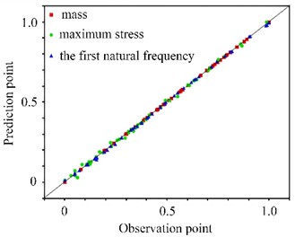
The scatter plot for verifying the fitting effect of the response surface function is shown in Fig. 18, which can be used to evaluate the prediction accuracy of the model for the three objectives of mass, maximum stress, and the first natural frequency. It can be seen that the predicted values are basically completely consistent with the true values, and all points will fall on the diagonal line. The degree of deviation from the diagonal line reflects the size of the model error. In the ideal state, the closer the points are to the diagonal line, the closer the predicted values are to the true values, and the higher the model accuracy. The farther the points deviate from the diagonal line, the greater the prediction deviation.
Fig. 18The scatter plot for verifying the fitting effect of the response surface function
Based on performance requirements, an optimized mathematical model is constructed as:
where and represent the minimum and maximum values of the design variables.
Due to the large number of optimization objectives, the Sequential Quadratic Programming (SQP) algorithm is prioritized for solving the optimization mathematical model. This algorithm is a classic method in the field of engineering optimization for handling constrained nonlinear optimization problems, and it is particularly suitable for scenarios involving continuous variables, smooth objective functions, and complex constraint combinations [21]. Since SQP utilizes the second-order derivative information (Hessian matrix) of the objective function, it achieves superlinear convergence, which is much faster than the gradient descent method that only uses first-order derivative information.
Through search-based computations, the optimization results are presented in Table 5. For the design variables, a targeted adjustment strategy was implemented. P1 was reduced from 16 mm to 13.3 mm, leveraging strength redundancy to achieve weight reduction. P2 was increased from 12 mm to 14.1 mm, compensating for stiffness loss. P3 was expanded from 180 mm to 209.8 mm, optimizing volume and stress distribution. P4 was decreased from 460 mm to 372.2 mm; while reducing weight, it controlled the overall stiffness, balancing mass, strength, and dynamic characteristics. In terms of mass, the initial value of 30,480 kg was reduced to 28,977.42 kg, achieving an approximate 4.93 % weight reduction. This aligns with the industry’s demand for cost reduction and efficiency improvement, enabling reduced transportation energy consumption or increased load capacity. For strength, the stress decreased from 3.953 MPa to 2.458 MPa, as shown in Fig. 19. Although it remains well below the allowable stress of structural steel, with existing strength redundancy, it ensures safety under extreme operating conditions. Regarding dynamic characteristics, the natural frequency increased from 7.26 Hz to 9.95 Hz, moving away from the low-excitation resonance range. This enhances anti-resonance capability and mitigates the risk of structural fatigue damage.
Table 5The result of optimization
Parameters | P1 / mm | P2 / mm | P3 / mm | P4 / mm | Y1 / kg | Y2 / MPa | Y3 / Hz | Weight loss rate / % |
Initial value | 16 | 12 | 180 | 460 | 30480 | 3.953 | 7.26 | 4.93 % |
Optimized value | 13.3 | 14.1 | 209.8 | 372.2 | 28977.42 | 2.458 | 9.95 |
Fig. 19The optimized stress under random vibration conditions

5. Conclusions
1) Compared with the previous multi-rigid-body dynamics research methods, the rigid-flexible coupling analysis incorporates the elastic deformation characteristics of the vehicle-mounted tank, which can accurately capture the dynamic interaction between the tank and the bogie, making the fluctuation of the center of mass acceleration more intense. However, due to the damping effect, the amplitude is relatively smaller, which is more in line with the actual situation. Modal analysis of the vehicle-mounted tank reveals complex vibration modes across different orders. The first-order mode is characterized by bending along the longitudinal axis, whereas higher-order modes exhibit more pronounced local vibrations. This insight is essential for predicting potential resonance and fatigue failure under dynamic loading conditions. Vibration response analysis demonstrates that the rigid-flexible coupling model effectively captures the distinct dynamic behaviors of the tank structure, with the flexible body showing greater sensitivity to high-frequency vibrations. Random vibration analysis under road excitation indicates that, although stress concentrations occur in critical regions, such as the central section of the tank and the connection between the tank and base frame, the overall structural integrity still satisfies strength requirements. Nevertheless, resonance risks within specific frequency bands (e.g., 5-15 Hz at side area and 0-5 Hz at middle area) must be carefully addressed in the design phase to mitigate fatigue damage.
2) The tank base structure was effectively optimized through the systematic process of design variable definition, correlation analysis, response surface function fitting, and optimization based on the Sequential Quadratic Programming algorithm. Targeted adjustments to the design variables, including the reduction of P1, increase of P2, expansion of P3, and reduction of P4, resulted in a significant 4.93 % weight reduction, accompanied by decreased stress levels and an increased natural frequency. This optimization successfully balanced the tank's mass, structural strength, and dynamic performance, fulfilling the industry’s demands for both economic efficiency and safety. The successful application of the SQP algorithm in solving multi-objective optimization problems demonstrates its capability to handle constrained nonlinear engineering problems, particularly those involving continuous variables, smooth objective functions, and complex constraint conditions. Compared with the previous single-objective optimization research, multi-objective optimization can generate a Pareto optimal solution set, where each solution is a non-dominated solution under different combinations of objectives. Therefore, it can achieve greater flexibility in the definition of optimization goals.
3) This research has made a contribution to the field by proposing a comprehensive approach for the dynamic analysis and structural optimization of vehicle-mounted tanks. This method bridges the gap between theoretical research and engineering practice, providing significant support for enhancing vehicle safety and promoting technological innovation in the automotive industry. Future research could focus on further improving the optimization model, taking into account more complex real-world conditions such as different road types, temperature variations, and material nonlinearity. Additionally, exploring the application of advanced optimization algorithms and machine learning techniques in the design optimization of vehicle-mounted tanks is expected to achieve a more efficient and intelligent design process.
References
-
A. Brown, “Analysis of structural parameters impacting vibration traits of heavy-duty truck fuel tanks,” Journal of Vehicle Engineering and Safety, Vol. 35, No. 2, pp. 189–205, Mar. 2024.
-
T. Schmidt, “Resonance-related hazards in aerospace fuel storage and their implications for ground-based transportation tanks,” International Journal of Transportation Safety, Vol. 18, No. 3, pp. 345–360, Jul. 2023.
-
K. Müller, “Vibration analysis of partially-filled cylindrical tanks under variable acceleration in road vehicles,” Vehicle System Dynamics, Vol. 60, No. 8, pp. 1123–1145, Aug. 2022.
-
L. Garcia, “The influence of vehicle-mounted tank structural design on vibration-induced fuel leakage risks,” Journal of Automotive Safety and Fuel Systems, Vol. 22, No. 4, pp. 567–583, Nov. 2021.
-
M. Johnson, “Optimizing support systems for vehicle-mounted tanks to mitigate vibration effects,” Transportation Engineering Journal, Vol. 146, No. 6, p. 04020, Jun. 2020.
-
K. Yamashita, “Vibration reduction technology using modal energy propagation analysis method for rigid-flexible coupled systems,” Journal of Vibration and Control, Vol. 30, No. 15, pp. 2255–2268, Aug. 2024, https://doi.org/10.1177/10775463241296415
-
M. Marano, “Stochastic multi-objective optimisation of exoskeleton structures for seismic retrofit,” Structural and Multidisciplinary Optimization, Vol. 64, No. 3, pp. 1890–1905, Jul. 2022.
-
R. Talebitooti, M. R. Zarastvand, and H. D. Gohari, “The influence of boundaries on sound insulation of the multilayered aerospace poroelastic composite structure,” Aerospace Science and Technology, Vol. 80, pp. 452–471, Sep. 2018, https://doi.org/10.1016/j.ast.2018.07.030
-
G. Flores, “Multi-objective optimization of vehicle suspension systems using NSGA-III,” Journal of Sound and Vibration, Vol. 534, p. 117144, 2023.
-
H. Lankarani, “Contact-impact dynamics of rigid-flexible coupled systems with clearance joints,” Multibody System Dynamics, Vol. 58, No. 2, pp. 177–205, Jun. 2023.
-
P. Ambrosio, “Multi-objective optimization of rotor-bearing systems for vibration suppression,” Mechanical Systems and Signal Processing, Vol. 170, p. 108850, Nov. 2022, https://doi.org/10.1016/j.ymssp.2022.108850
-
S. He, J. He, X. Guo, T. Ueda, and Y. Wang, “Detection of CFRP-concrete interfacial defects by using electrical measurement,” Composite Structures, Vol. 295, p. 115843, Sep. 2022, https://doi.org/10.1016/j.compstruct.2022.115843
-
M. R. Zarastvand, M. Ghassabi, and R. Talebitooti, “Acoustic insulation characteristics of shell structures: a review,” Archives of Computational Methods in Engineering, Vol. 28, No. 2, pp. 505–523, Dec. 2019, https://doi.org/10.1007/s11831-019-09387-z
-
R. Talebitooti and M. R. Zarastvand, “Vibroacoustic behavior of orthotropic aerospace composite structure in the subsonic flow considering the Third order Shear Deformation Theory,” Aerospace Science and Technology, Vol. 75, pp. 227–236, Apr. 2018, https://doi.org/10.1016/j.ast.2018.01.011
-
J. Yin et al., “Research on lightweight rail vehicle body based on sensitivity analysis,” Journal of Engineering and Technological Sciences, Vol. 56, No. 3, pp. 353–366, Jun. 2024, https://doi.org/10.5614/j.eng.technol.sci.2024.56.3.4
-
Z. Men, D. Gong, K. Zhou, Y. Chen, and J. Zhou, “Unsupervised domain adaptation method for bearing fault diagnosis assisted by twin data under extreme sample scarcity,” Mechanical Systems and Signal Processing, Vol. 239, No. 1, p. 113359, Oct. 2025, https://doi.org/10.1016/j.ymssp.2025.113359
-
T. Mazilu, M. Dumitriu, Sorohan, M. A. Gheți, and I. I. Apostol, “Testing the effectiveness of the anti-bending bar system to reduce the vertical bending vibrations of the railway vehicle carbody using an experimental scale demonstrator,” Applied Sciences, Vol. 14, No. 11, p. 4687, May 2024, https://doi.org/10.3390/app14114687
-
R. Talebitooti, M. Zarastvand, and H. Darvishgohari, “Multi-objective optimization approach on diffuse sound transmission through poroelastic composite sandwich structure,” Journal of Sandwich Structures and Materials, Vol. 23, No. 4, pp. 1221–1252, Jun. 2019, https://doi.org/10.1177/1099636219854748
-
R. Talebitooti and M. R. Zarastvand, “The effect of nature of porous material on diffuse field acoustic transmission of the sandwich aerospace composite doubly curved shell,” Aerospace Science and Technology, Vol. 78, No. 1, pp. 157–170, Jul. 2018, https://doi.org/10.1016/j.ast.2018.03.010
-
A. Fiore, “Modal analysis and structural optimization of composite LNG tanks,” Applied Acoustics, Vol. 201, p. 10790, Sep. 2023.
-
R. Acciani, “Multi-objective optimization of vehicle suspension systems using kriging models,” Applied Soft Computing, Vol. 139, p. 10971, Sep. 2023.
About this article

The paper is supported by provincial scientific research projects (2023YFG1066).
The datasets generated during and/or analyzed during the current study are available from the corresponding author on reasonable request.
The authors declare that they have no conflict of interest.
