Application of improved support vector machine regression analysis for medium- and long-term vibration trend prediction

1. Introduction

The performance of aircraft engine decreased through time, and it is important to effectively evaluate and predict this performance. To do so, the change rate of vibration parameters need to be analyzed to help better understand the vibration trend, discover potential faults, estimate the remaining useful life of critical components, and reveal the recession trend of the performance of aircraft engine [1]. Accurate trend forecast of the engine performance is essential, which could help determine whether the engine would be operable in the near future. Engine performance checking and potential fault diagnosis need to be done regularly, and methods for predicting performance trends of relevant applications need to be updated to increase the diagnostic accuracy, reduce the occurrence of false alarms and improve flight safety [2]. Furthermore, recorded data could be further processed using more complicated algorithms and models so that early detection of abnormal conditions, including unbalance, wear, tear and rubbing fault can be realized, and corresponding actions can be taken in a timely manner.

The existing prediction methods can be divided into qualitative prediction and quantitative prediction. Compared to the latter, the former often fails to provide accurate predictions. The latter can be further divided into timing sequence relationship prediction and causality prediction. Also, it can be specifically classified into regression analysis prediction, timing sequence prediction, Markov chain prediction, grey prediction, Bayes network prediction and neural network prediction [3], among which timing sequence prediction, Markov chain prediction, grey prediction and neural network prediction belong to timing sequence relationship prediction category, whereas Bayes network prediction and regression analysis prediction belong to causality prediction category. In general, timing sequence relationship prediction is widely applied because timing sequence data are easy to collect. In some cases, however, further analysis with causality prediction applied is required [4], and the selection of time lags for time series forecasting by fuzzy inference systems, for which optimal non-uniform attractors are embedded in the multidimensional delay phase space, is especially needed [5]. Recently, a new model was proposed to predict rain rate time series in tropical rainforests [6], and time series prediction techniques have been applied to significantly reduce the radio use and energy consumption of wireless sensor nodes performing periodic data collection tasks [7]. A computational framework was used to generate daily temperature maps using time-series method based on temperature measurements from the national network of meteorological stations [8]. Because each prediction method has its own advantages and disadvantages, the best predictive method needs to be selected in accordance with different modes of faults and features.

Based on the predictive operation conditions and fault variation properties of aircraft engine, this study tested the applicability of nonlinear predictive method in predicting the operational vibrating faults of aircraft engine in a long-term scale. Support vector regression (SVR) was applied to evaluate whether the predicted vibrating values were in accordance with the technical requirements of the predictive technology used for evaluating aircraft engine operational conditions. This study proposed that improved support vector regression algorithms with smooth operators included could increase the predictive power and accuracy of both medium- and long-term trend. Moreover, the constrained quadratic optimization problem could be converted to unconstrained optimization problem, and model verification was done using historical vibration data. The results showed that even vibrating values in a longer interval could be predicted with high accuracy.

2. Improvement of the support vector regression algorithm

Support vector machine was initially used to solve classification problems. Afterwards, its application was extended to the regression field [9]:

In the above set, $x_i$ is a $n$-dimensional coordinate and $y_i$ is the corresponding value of $x_i$. In any regression analysis, a function needs to be defined to predict the value of any given point $\omega$. Meanwhile, the error of regression model needs to be minimized [10]. In a linear regression model, regression function is defined as follows:

Nuclear technology is of great importance in support vector machine analysis, and, nonlinear problems should be converted into linear problems by adopting methods commonly used in nuclear technology to solve regression problems [11]. A nonlinear mapping $\Phi$ is adopted to map the data in a high-dimensional feature space $G$. A linear approximation is then applied to minimize the expected risk function as follows:

In the above formula, $\omega$ is the generalized parameter in the high-dimensional feature space $G$, $(·)$ is the inner product and $b$ is the constant term.

Function approximation is equivalent to minimize the structure risk function $R_{reg}\left[f\right]$:

In the above formula, $R_{emp}$ is the empirical risk and $l(·)$ is the loss function, representing the deviation between $y$ and $C$ [12]. $\epsilon$ is used to represent the error of regression model:

Then empirical risk is:

In the above formula, $C$ is a positive parameter defined in advance. When the difference between the predictive value and the observed value is less than $\epsilon$, it is considered that no loss is produced. $R_{emp}^{\epsilon }\left[f\right]$ is used to minimize the formula 2, with both the training error and model complexity controlled. Similar to the mentality of classification problem, this problem could be converted into an optimization problem [13]:

In the above formula, ${\xi }_i^{*}$, ${\xi }_i$ is the slack variable when the difference between the predictive value and observed value is larger than $\epsilon$, thus allows some points functioning as outliers far away from predictive functions [14]. $C$ is the punishment variable, which is applied when the difference between the predictive value and observed value is larger than $\epsilon$. Similar to classification problems, Lagrangian function could be established to calculate the extreme points, get dual problem and finally calculate weight vector and excursion.

Formula (7) can be converted into the following formula by adopting kernel function $K(x_i,x_j)=\Phi \left(x_i\right)·\Phi \left(x_j\right)$:

Nonlinear mapping with convex quadratic programming is represented as:

Clearly, how to select design parameters $C$ and $\epsilon$ is an essential question for support vector regression model analysis. The value of $C$ determines the penalty to samples when training errors exceed $\epsilon$. The selection of $C$ exerts great influence on the generalization ability of the system, and the value of $\epsilon$ directly influences the predictive accuracy. If a small value of $\epsilon$ is selected, the requirement for regression predictive accuracy will be high and the quantity of support vector machines will increase [15]; by contrast, if a large value of $\epsilon$ is selected, regression predictive accuracy will decrease. Therefore, the selection process of $C$ and $\epsilon$ is extremely complicated, although how to select these parameters in order to attain a good regression result remains unsolved in practice.

As support vector regression method deals with a constrained quadratic programming problem, the high computational complexity could lead to a low computing speed. Also, this method requires large computing memory and thus its use would be limited, especially for massive data. In order to improve the computing peed of support vector regression algorithm and decrease its training complexity, a methodical improvement of support vector regression is necessary. By adopting the smoothing method, the constrained quadratic optimization problem in traditional support vector regression could be converted to unconstrained convex quadratic optimization problem, with the loss function converted to an $\epsilon$ insensitive quadratic function. For convenience, this conversion process in support vector machine regression is represented as follows:

Institute the regular factor $C$ with $\frac{C}{2}$ and add another term $\frac{b^2}{2}$, formula (10) becomes:

Apply the following conversion:

Define the following function ${\left(u\right)}_{+}=\mathrm{m}\mathrm{a}\mathrm{x}\{u,0\}$ and make${\xi }_i={\left(z_i\right)}_{+}$, ${\xi }_i^{*}={\left(z_i^{*}\right)}_{+}$. Also, formula (11) can be converted into the following unconstrained quadratic optimization problem:

Formula (13) represents an unconstrained convex quadratic optimization problem. Because the target function is not twice differentiable, we define a strictly convex and infinitely differentiable smooth function $p\left(u,a\right)\text{=}\frac{1}{\alpha }\mathrm{l}\mathrm{n}\left(1+e^{\alpha u}\right),\alpha >0$ and institute ${\left(u\right)}_{+}$ with $p(u,a)$. Therefore, a smooth support vector regression objective function is represented as follows:

3. Trend prediction simulation analysis based on SVR

To compare the effectiveness of artificial neural network and improved support vector regression, both RBF neural network and support vector regression algorithms are programmed under MatlabR2009a environment [16]. A continuous function model is given as following:

$y=\mathrm{c}\mathrm{o}\mathrm{s}\left(e^x\right)+\mathrm{s}\mathrm{i}\mathrm{n}\left(x\right)$, $x\in [2,\mathrm{}4]$.

The sampling interval is 0.1, with 21 sample data produced. In RBF neural network model, the network training is set as 1000 times, and the minimum error is set as 0.002. In support vector regression model, RBF kernel function is adopted, with kernel parameter $\sigma =$ 0.07 and model parameters $C=$ 600, $\epsilon =$ 0.02. The regression result of the continuous function model is shown in Fig. 1.

Fig. 1Regression results derived from both SVR and RBF

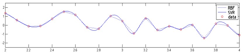
It can be seen form Fig. 1 that the predictive curves and actual curves of the two models coincide with each other with small predictive error and high regression accuracy.

The main problem of neural network, however, lies in that the regression curve is not smooth enough. As can be seen from Fig. 1, the regression curve (the dotted line) is just a direct connection among sample points and thus yields unsatisfactory results [17]. By contrast, the regression curve of SVR (the solid line) coincides well with the realistic curve of the continuous function model with better regression accuracy.

Although neural network has a strong capability of nonlinear approximation, it focuses exclusively on error minimization but loses the generalization property and thus is limited for time series analysis. By contrast, support vector regression algorithm has higher generalization ability, and thus provides a better fit of the data.

4. Predictions of aircraft engine vibrations using improved SVR models

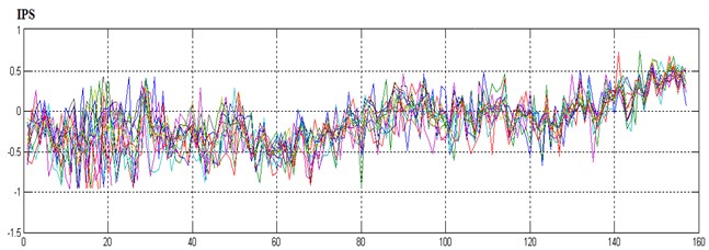
Vibration data were measured for eight flights in 155 days so that the dataset could be represented in a matrix of 8×155. The time sequence of the dataset was shown in Fig. 2.

Fig. 2Tendency chart of all vibration data

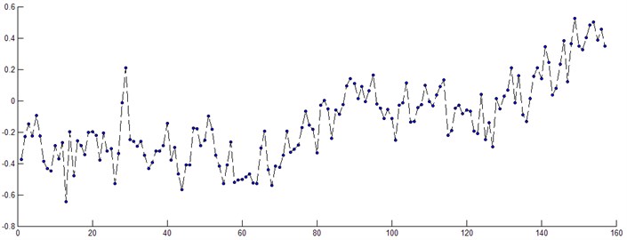
Further analysis and denoising process were applied to the collected vibration data. The maximum value of vibration intensity was obtained to form an unvaried time sequence. The sequence included 155 data points, as shown in Fig. 3. These data points were further divided into two parts, with 130 data points used for training models and related optimizing model parameters, and the rest 25 data points used for model evaluation and validation.

Fig. 3Single variable sequence of the vibration intensity

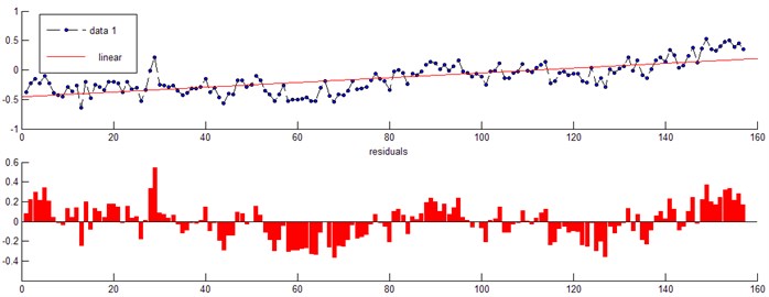
In the first step, linear function was applied and corresponding predictive trend was shown in Fig. 4. It could be seen that the increasing trend of total vibration was obvious.

Obviously, when linear function was applied, the displayed trend was simple and clear, and related fault problems were easy to identify. However, one obvious disadvantage of linear function was its high predictive error. In Fig. 4, we could see that the difference between the predictive value and practical value was large with an average error of 7.32 %.

BP algorithm is commonly adopted for artificial neural network. The predictive aim error for setting BP neural network is 0.001 and network training is operated 2000 times. However, BP network fails to achieve the target value set after network training is operated more than 2000 times. At that stage, the owe training problem occurs. After network training is operated for 3573 times, the network stops training with the final training error as 0.049.

Fig. 4Linear prediction trend chart and error analysis

The prediction trend chart is shown in Fig. 5. Obviously, the predictive curve of BP algorithm matches the real variation trend perfectly, but it brings other problems, such as longer calculation time, larger memory space requirement and lower prediction accuracy.

Radial kernel function was adopted for SVR prediction and the parameter settings were as follows: $C=$ 1200, $\sigma =$ 1.5, $\epsilon =$ 0.005. All predictive values were shown in Fig. 6.

SVR was applied to the same time series dataset (i.e., 130 data points), with extremely small error gained from the training model, and the remaining 25 data points were used to test prediction accuracy of SVR model (the predictive average relative error was 1.327 %). The results showed that SVR was well applied to nonlinear time series for accurate prediction in a long-term scale. Also, it demonstrated the effectiveness of the predictive method proposed in this study when used for predicting the performance of aircraft engine.

Fig. 5Neural network prediction trend chart and error analysis

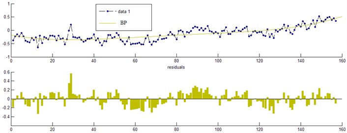
Fig. 6Prediction trend chart and error analysis of SVR model

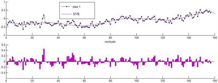
Fig. 7 showed the comparison chart of errors in the engine predictive results using both SVR and BP. It could be seen from the chart that the prediction error using SVR was smaller then that using BP, with the average predictive relative error 3.573 % smaller for the former compared to that of the latter.

Fig. 7Comparison between predictive errors of neural network and SVR

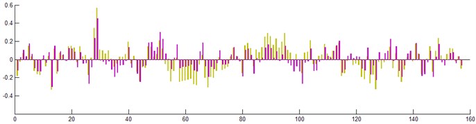
Compared with neural network, SVR prediction model has smaller error and stronger generalization ability. As neural network unilaterally minimizes errors when it is used to deal with practical dataset with noises, over fitting or over learning could easily occur, which would decrease the prediction accuracy of neural network. By contrast, SVR reflects the obvious features that support vector machine networks and help compromise structural risks. Since the time series variation rule of the predictive values and the real values are approximately the same, time series analysis could be widely applied to simulate the real process.

5. Conclusions

Support vector algorithm could be used to solve problems associated with quadratic programming, such as slow running speed and large storage space requirement. Smoothing operators are introduced in this study to improve model fitness and decrease the complexity of training. Simulation tests show that smoothing support vector machine has fast operation speed and high predictive accuracy, and is very fit for eary detection of the performance of aircraft engines with complicated vibration patterns.

The effectiveness of SVR method depends on insensitive factor $\epsilon$, penalty factor $C$, the type of kernel function and its parameter $S$. The interplay between these parameters is complicated, and a proper matching could help improve prediction accuracy.

However, trend analysis method has its disadvantages. For example, it has high requirements for data collections. Also, it can only detect engine faults rather than reveal the causes of these faults. Furthermore, it is insensitive to detect some types of engine faults. Therefore, further studies should address above mentioned questions.