Identification of parameter matrices using estimated FRF variation

Kim, Jin Bong; Eun, Hee-Chang

Journal of Vibroengineering

Browse Journal

Submit article

Published: 31 March 2013

Check for updates

Identification of parameter matrices using estimated FRF variation

Jin Bong Kim¹

Hee-Chang Eun²

^{1, 2}Department of Architectural Engineering, Kangwon National University, Chuncheon, Korea

Corresponding Author:

Hee-Chang Eun

Cite the article Download PDF

Downloads 1192

Abstract

This study presents an analytical method to predict the dynamic parameters of actual structure from measured FRF (Frequency Response Function) data. The inconsistency due to modeling errors between the actual structure and the finite element model exists. The number of measured data is less than the one of a full set of dofs and should be expanded to estimate the parameters. Considering that the stiffness and mass matrices are related with the real part of the expanded FRF data and the damping matrix with the imaginary part, the variation in the parameter matrices is evaluated. A numerical example evaluates the appropriateness of the proposed method.

1. Introduction

The FRFs have been used directly to update condensed analytical models for obtaining the proper model. A single FRF measured at several frequencies, along with a correlated analytical model of the structure in its original state, is used for updating structural parameters. However, it’s impossible to get the data of a full set of dofs and the sparse data should be expanded to get the information of the whole system.

There have been many attempts to update the unknown physical parameters directly from the FRFs [1]. It has been reported [2] that FRF data provide more information than modal data, as the latter are extracted from a very limited frequency range related to resonance. Friswell and Penny [3] proposed an approach to reduce the model order so that the stated estimation process reduces to a least squares problem based on the FRFs. Fanning and Carden [4] presented a method for detecting added mass in structural systems from a single FRF measured at several frequencies in an identification algorithm. Cha and Tuck-Lee [5] developed approaches to update mass and stiffness matrices based on two sets of measured frequency response data. Kwon and Lin [6] proposed a frequency selection method for efficient FRF-based model updating. Lin and Zhu [7] developed model updating methods to identify mass, stiffness, and damping matrices of a damaged dynamic system based on the FRF method. Phani and Woodhouse [8] identified parameter matrices of viscous damping models based on measured FRFs. They compared matrix methods using a measured FRF matrix and modal methods using modal parameters. Inverting the FRF matrix to the dynamic stiffness matrix and comparing their real and imaginary parts with parameter matrices, Lee and Kim [9] identified damping characteristics of the system in matrix forms directly from its measured FRFs. Fritzen [10] proposed an analytical method to describe the parameter matrices by minimizing the error of a dynamic stiffness matrix and its inverse, and an identity matrix. Utilizing FRF data measured at specific positions, with dofs less than that of the system, as constraints to describe a damaged system, Rahmatalla et al. [11] predicted parameter matrices such as mass, stiffness and damping matrices of the system, and provided a damage identification method from their variations. Changes of FRF of a structure are correlated to changes of the stiffness and mass through damage sensitivity equations which have been derived using the change of eigenvectors and measured natural frequencies of damaged structures. Pascual et al. [12] presented a model updating method to avoid the numerical difficulties induced by the discontinuities in the FRFs. Esfandiari et al. [13], [14] provided a structural model updating technique using measured FRF data and measured natural frequencies of the damaged structure without any expansion of the measured data or reduction of the finite element model. When solving damage sensitivity equations by the least square method, they estimated the mass, stiffness and damping properties.

This study begins with the expansion of a few measured FRF data to a full set of dofs and presents the mathematical form of the updated FRF matrix. And this work presents an analytical method to estimate the dynamic parameters from the FRF variation between the actual system and the finite element model. The parameters include the stiffness, mass and damping matrices and are estimated from the variation in the real and imaginary parts of the expanded FRFs. A numerical example illustrates the appropriateness of the proposed method.

2. Formulation

2.1. Expansion of FRF data

Structures can be modeled as discrete systems with the assumption of homogeneous and uniform systems without any defect. And the finite element analysis can be used to approximate the dynamic behavior of the systems. Using the finite element method, the dynamic equation for a damped dynamic system is a system of second-order differential equations. The dynamic response of a structure in the time-domain which is assumed to be linear and approximately discretized for $n$ dofs can be described by the equations of motion:

1

M \ddot{u} + C \dot{u} + K u = f (t),

where $M$ , $C$ , and $K$ denote the $n \times n$ analytical mass, damping, and stiffness matrices, respectively, $u = {[\begin{matrix} u_{1} & u_{2} & \dots & u_{n} \end{matrix}]}^{T},$ and $f (t)$ is the $n \times 1$ excitation vector.

In the frequency-domain methods each component is described by frequency-dependent data. A relationship between FRF and modal parameters for successful modal testing is established by inserting $u = U e^{j Ω t}$ and $f = F e^{j Ω t}$ into Eqn. (1). Then expressing it in the frequency-domain, it follows that:

2a

(K - Ω^{2} M + j Ω C) U (Ω) = F (Ω),

where $Ω$ denotes the excitation frequency, $F$ is an external force vector with an element being unit and all other elements zeros, and $j = \sqrt{- 1}$ . The relation of Eqn. (2a) for the actual structure can be written by:

2b

(K^{*} - Ω^{2} M^{*} + j Ω C^{*}) U^{*} (Ω) = F (Ω),

where $M^{*}$ , $C^{*}$ and $K^{*}$ represent the mass, damping and stiffness matrices of the actual structure, respectively, and $U^{*}$ is the modal displacement vector of the actual structure. Using the FRF matrix, the responses of the structure, described by $U (Ω)$ and $U^{*} (Ω)$ to an external excitation, described by $F (Ω)$ , are given by:

3a

U (Ω) = H (Ω) F (Ω),

3b

U^{*} (Ω) = H^{*} (Ω) F (Ω),

where $H (Ω) = {(K - Ω^{2} M + j Ω C)}^{- 1}$ is the FRF matrix of the finite element model, whose elements can be the receptances. And $H^{*} (Ω) = {(K^{*} - Ω^{2} M^{*} + j Ω C^{*})}^{- 1}$ is the FRF matrix of the actual structure.

Expressing the FRF variation between the actual system and the finite element model by $Δ H,$ the actual FRF matrix $H^{*} (Ω)$ can be established as:

4

H^{*} (Ω) = H (Ω) + Δ H .

The elements in the FRF matrix are derived as follows. Equations (2) can be transformed as:

5a

(- Ω^{2} + 2 j ξ_{i} ω_{i} Ω + ω_{i}^{2}) U (Ω) = F (Ω), i = 1,2, \dots, n,

5b

(- Ω^{2} + 2 j ξ_{i}^{*} ω_{i}^{*} Ω + ω_{i}^{* 2}) U^{*} (Ω) = F (Ω), i = 1,2, \dots, n,

where $ω_{i}$ and $ξ_{i}$ denote circular natural frequency and damping ratio corresponding to the i-th mode, respectively. And $ω_{i}^{*}$ and $ξ_{i}^{*}$ denote circular natural frequency and damping ratio of the actual structure, respectively. Applying modal transformation, the real eigenvalues and eigenvectors lead to the representation of the FRF matrices for an excitation frequency $Ω$ :

6a

H (Ω) = \sum_{i = 1}^{n} \frac{φ_{i} φ_{i}^{T}}{ω_{i}^{2} - Ω^{2} + 2 j ξ_{i} ω_{i} Ω},

6b

H^{*} (Ω) = \sum_{i = 1}^{n} \frac{φ_{i}^{*} φ_{i}^{* T}}{ω_{i}^{*} - Ω^{2} + 2 j ξ_{i}^{*} ω_{i}^{*} Ω},

where $φ_{i}$ and $φ_{i}^{*}$ are the i-th mode shape vectors of the finite element model and actual structure, respectively. For the case of a displacement response at station $p$ and a disturbing force at station $q$ , the numerical frequency response can be constructed as:

7a

H_{p, q} (Ω) = \sum_{i = 1}^{n} \frac{ϕ_{i, p} ϕ_{i, q}}{ω_{i}^{2} - Ω^{2} + 2 j ξ_{i} ω_{i} Ω},

7b

H_{p, q}^{*} (Ω) = \sum_{i = 1}^{n} \frac{ϕ_{i, p}^{*} ϕ_{i, q}^{*}}{ω_{i}^{* 2} - Ω^{2} + 2 j ξ_{i}^{*} ω_{i}^{*} Ω},

where $ϕ_{i, p}$ denotes the pth element of the vector $ϕ_{i}$ .

It is impossible to experimentally collect all FRF data corresponding to the full dofs and to explicitly match the actual structure with the analytical model. It indicates that the physical parameters should be corrected to describe the actual system. To update the parameters it is necessary to expand the measured data or to reduce the dofs of the dynamic system.

Assume that the FRFs of the system were measured at $m (m < n)$ different positions of the $r (r < n)$ set of unitary excitations. The measured $m \times n$ FRF matrix and the response vector have the relationship of:

8

U_{m}^{*} (Ω) = A U^{*} = H_{m}^{*} (Ω) F (Ω),

where $A$ is an $m \times n$ Boolean matrix to define the measured locations. The subscripts m and u represent the measured and unmeasured dofs, respectively, and $U_{m}^{*}$ and $U_{u}^{*}$ represent the $m \times r$ and $(n - m) \times r$ measured and unmeasured displacement matrices, respectively, and $U^{*} = {[\begin{matrix} U_{m}^{*} \\ U_{u}^{*} \end{matrix}]}_{n \times r}$ . $F$ is the $n \times r$ excitation matrix, $F = [\begin{matrix} F_{1} & F_{2} & \dots & F_{r} \end{matrix}]$ where $F_{i}$ denotes the i-th unitary vector of excitation, and $F = {[\begin{matrix} F_{m} \\ F_{u} \end{matrix}]}_{n \times r}$ . And $F_{m}$ and $F_{u}$ are the $m \times r$ and $(n - m) \times r$ force matrices corresponding to the measured and unmeasured locations. $H_{m}^{*} (Ω)$ denotes the $m \times n$ measured FRF matrix corresponding to the $m$ rows in the FRF matrix.

The measured FRF matrix relation of Eqn. (8) can be regarded as constraint conditions to describe the FRF matrix of the whole system. Utilizing the generalized inverse method shown in Ref. [15], the updated dynamic equation of Eqn. (3b) can be explicitly derived. The updated response vector $U^{*}$ is derived as:

9

U^{*} = U + Δ U,

10

Δ U = [H^{1 / 2} {(A H^{1 / 2})}^{+} (H_{m}^{*} - A H)] F,

where the superscript ‘+’ indicates the Moore-Penrose inverse. $Δ U$ indicates the variation in the displacement. The dynamic parameters can be grasped by investigating the displacement variation. And the updated FRF matrix can be written in the form of Eqn. (4) and the variation in the FRF matrix can be predicted by:

11

Δ H = [H^{1 / 2} {(A H^{1 / 2})}^{+} (H_{m}^{*} - A H)] .

The variation in the parameter matrices can be explained by the FRF variation of Eqn. (11). The updated FRF matrix obtained from a few measured FRF data can be written by:

12

H^{*} = H + H^{1 / 2} {(A H^{1 / 2})}^{+} (H_{m}^{*} - A H) .

The accuracy of the FRF matrix depends on the number of measured FRF data. The FRF variation $Δ H$ will be more accurately calculated with the increase in the number. Its effectiveness will be investigated by establishing the updated parameter matrices.

2.2. Update of parameter matrices

The parameter matrices are calculated by the following process. Post-multiplying both sides of $H^{*} (Ω) = {(K^{*} - Ω^{2} M^{*} + j Ω C^{*})}^{- 1}$ by $(K^{*} - Ω^{2} M^{*} + j Ω C^{*})$ , it can be expressed by:

13

H^{*} (K^{*} - Ω^{2} M^{*} + j Ω C^{*}) = I,

and inserting $H^{*} = H_{r e}^{*} + H_{i m}^{*}$ , $K^{*} = K + Δ K$ , $M^{*} = M + Δ M$ and $C^{*} = C + Δ C$ into Eqn. (13), and arranging the result, the variation in the parameters can be rewritten by:

14

[\begin{matrix} H_{r e}^{*} & - Ω^{2} H_{r e}^{*} & - Ω H_{i m}^{*} \\ H_{i m}^{*} & - Ω^{2} H_{i m}^{*} & Ω H_{r e}^{*} \end{matrix}] [\begin{matrix} Δ K \\ Δ M \\ Δ C \end{matrix}] = [\begin{matrix} I - H_{r e}^{*} K + Ω^{2} H_{r e}^{*} M + Ω H_{i m}^{*} C \\ - H_{i m}^{*} K + Ω^{2} H_{i m}^{*} M - Ω H_{r e}^{*} C \end{matrix}] .

Expanding Eqn. (14) in a specific frequency range of ${[\begin{matrix} Ω_{1} & Ω_{2} & \dots & Ω_{m - 1} & Ω_{m} \end{matrix}]}^{T},$ it is expressed as:

15

[\begin{matrix} Δ K \\ Δ M \\ Δ C \end{matrix}] = {[\begin{matrix} H_{r e}^{*} (Ω_{1}) & - Ω_{1}^{2} H_{r e}^{*} (Ω_{1}) & - Ω_{1} H_{i m}^{*} (Ω_{1}) \\ H_{i m}^{*} (Ω_{1}) & - Ω_{1}^{2} H_{i m}^{*} (Ω_{1}) & Ω_{1} H_{r e}^{*} (Ω_{1}) \\ ⋮ & ⋮ & ⋮ \\ H_{r e}^{*} (Ω_{m}) & - Ω_{m}^{2} H_{r e}^{*} (Ω_{m}) & - Ω_{m} H_{i m}^{*} (Ω_{m}) \\ H_{i m}^{*} (Ω_{m}) & - Ω_{m}^{2} H_{i m}^{*} (Ω_{m}) & Ω_{m} H_{r e}^{*} (Ω_{m}) \end{matrix}]}^{+}

∙ [\begin{matrix} I - H_{r e}^{*} (Ω_{1}) K + Ω_{1}^{2} H_{r e}^{*} (Ω_{1}) M + Ω_{1} H_{i m}^{*} (Ω_{1}) C \\ - H_{i m}^{*} (Ω_{1}) K + Ω_{1}^{2} H_{i m}^{*} (Ω_{1}) M - Ω_{1} H_{r e}^{*} (Ω_{1}) C \\ ⋮ \\ I - H_{r e}^{*} (Ω_{m}) K + Ω_{m}^{2} H_{r e}^{*} (Ω_{m}) M + Ω_{m} H_{i m}^{*} (Ω_{m}) C \\ - H_{i m}^{*} (Ω_{m}) K + Ω_{m}^{2} H_{i m}^{*} (Ω_{m}) M - Ω_{m} H_{r e}^{*} (Ω_{m}) C \end{matrix}] .

The variation in the parameter matrices can be estimated by Eqn. (15). It can be observed that the variation can be predicted by the expansion of a few measured FRFs and Eqn. (15). The accurate estimation of the updated FRF matrix helps the determination of the exact parameter matrices of the structure. It indicates that the effectiveness of the proposed method requires enough number of measured FRF data.

3. Application

Consider the estimation of the parameter matrices of a plane truss structure model shown in Fig. 1. The nodal points and the members are numbered as shown in the figure. The truss is composed of 15 nodes and 33 members. Corresponding to each pair of nodal displacement components $(u_{i}, v_{i})$ is expressed by a set of forces $(H_{i}, V_{i})$ . All members have elastic modulus of 200 GPa, cross-sectional area of 2.5×10^-3 m², and density of 7860 kg/m³.

Fig. 1A planar truss structure

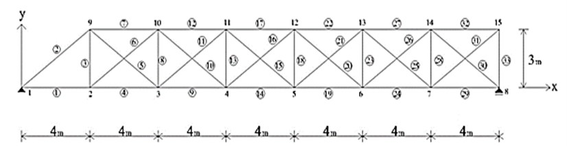
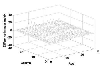
For this application, we assumed that the actual structure includes 0-23 % manufacturing errors in all truss members. They were randomly given for this numerical experiment. The physical parameter matrices are updated using the proposed method and measured FRF data. Assume that the FRF matrix of the first 15 rows corresponding to the 1st to 8th node was measured by numerical simulation. The FRF matrix was updated with the measured noise-free FRF data in the range of 8.4-8.8 Hz in steps of 0.02 Hz. Figure 2 exhibits the difference in the parameter matrices between before and after the correction by this proposed method. The difference comes from the inconsistency with the actual parameter matrices that cannot be expressed by the finite element model. The parameter update should be performed for solving such inconsistency. The parameter should be corrected by a few measurement data only because it is difficult to collect all measurement data on the full set of dofs. Figure 3 displays the difference between the actual and the updated parameter matrices. The difference is due to the neglecting of the half of FRF data, which do not provide all information on the actual truss structure. It is shown that the proposed method rarely describes the accurate parameter matrices and its accuracy will be improved with the increase in the number of measurements.

Table 1 compares the natural frequencies of the 1^st to 5^th mode. In the table, the “Initial” represents the numerical results of the finite element model, the “Actual” is the ones of the actual truss including the manufacturing errors and the “After correction” denotes the ones corrected by this proposed method. It is exhibited that the proposed method properly describes the global characteristics of the structure despite of the inconsistency of the parameters of the truss members.

Table 1Natural frequencies of initial, actual and corrected structure (rad./sec.)

Mode number	1st	2nd	3rd	4th	5th
Initial	54.6	161.8	224.5	412.5	569.2
Actual	54.9	163.1	225.2	411.2	571.7
After correction	54.9	163.0	225.1	411.0	570.2

Fig. 2Difference in parameter matrices between before and after correction: (a) stiffness matrix, (b) mass matrix, (c) damping matrix

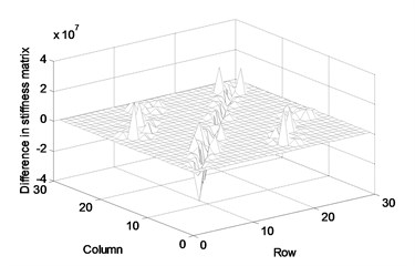
a)

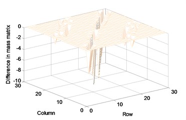
b)

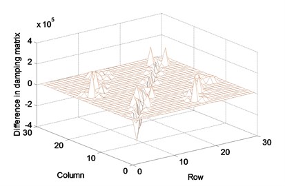
c)

Fig. 3Difference between actual and numerically derived parameter matrices: (a) stiffness matrix, (b) mass matrix, (c) damping matrix

(a)

(b)

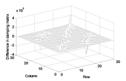
(c)

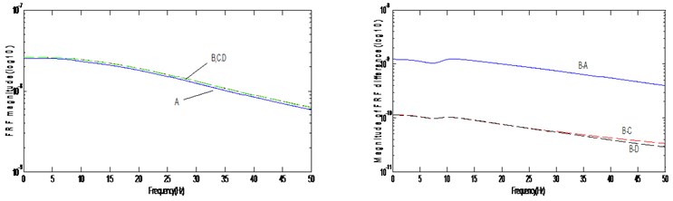
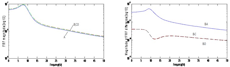
Fig. 4FRF magnitude and FRF difference: (a) H*(27,27) (b) H*(28,28)

(a)

(b)

Figure 4 exhibits the FRF magnitudes of $H^{*} (27,27)$ and $H^{*} (28,28)$ corresponding to the horizontal and vertical components at node 13. In the plots, “A” represents the FRF of the finite element model, “B” the actual structure, “C” the estimated FRF obtained by Eqn. (12), and “D” the FRF rebuilt by the updated parameter matrices. The FRF figures were plotted in the range of 0.01-50 Hz in steps of 0.02 Hz. The figures exhibit some difference between the actual truss, B, and the finite element model, A. And it is observed that the C and D plots coincide with the actual plot B. It indicates that the proposed method properly describes the FRF curves although it rarely provides the accurate parameter matrices. It can be overcome by increasing the number of the measured FRF data.

4. Conclusions

This study provided the analytical method to describe the inconsistent physical parameters between the actual structure and the finite element model. Beginning with the measured FRF for less than the full set of dofs, this work predicted the updated FRF matrix. And the stiffness and mass matrices were estimated from the real part of the expanded FRF data and the damping matrix was predicted from the imaginary part. The proposed method properly describes the FRF curves although it rarely provides the accurate parameter matrices. It can be overcome by increasing the number of the measured FRF data.

References

Mottershead J. E., Stanway R. Identification of structural vibration parameters by using a frequency domain filter. Journal of Sound and Vibration, Vol. 109, 1986, p. 495-506.

Search CrossRef
Lee U., Shin J. A frequency response function-based structural damage identification method. Computers & Structures, Vol. 80, 2002, p. 117-132.

Search CrossRef
Friswell M. I., Penny J. E. T. Updating model parameters from frequency domain data via reduced order models. Mechanical Systems and Signal Processing, Vol. 4, 1990, p. 377-391.

Search CrossRef
Fanning P. J., Carden E. P. Experimentally validated added mass identification algorithm based on frequency response functions. Journal of Engineering Mechanics, Vol. 130, 2004, p. 1045-1051.

Search CrossRef
Cha P. D., Tuck-Lee J. P. Updating structural system parameters using frequency response data. Journal of Engineering Mechanics, Vol. 126, 2000, p. 1240-1246.

Search CrossRef
Kwon K. S., Lin R. M. Frequency selection method for FRF-based model updating. Journal of Sound and Vibration, Vol. 278, 2004, p. 285-306.

Search CrossRef
Lin R. M., Zju J. Model updating of damped structures using FRF data. Mechanical Systems and Signal Processing, Vol. 20, 2006, p. 2200-2218.

Search CrossRef
Phani A. S., Woodhouse J. Viscous damping identification in linear vibration. Journal of Sound and Vibration, Vol. 303, 2007, p. 475-500.

Search CrossRef
Lee J. H., Kim J. Identification of damping matrices from measured frequency response functions. Journal of Sound and Vibration, Vol. 240, 2001, p. 545-565.

Search CrossRef
Fritzen C. P. Identification of mass and stiffness matrices of mechanical systems. Journal of Vibration and Acoustics, Vol. 108, 1986, p. 9-16.

Search CrossRef
Rahmatalla S., Eun H. C., Lee E. T. Damage detection from the variation of parameter matrices estimated by incomplete FRF data. Smart Structures and Systems, Vol. 9, 2012, p. 55-70.

Search CrossRef
Pascual R., Schalchli R., Razeto M. Damping identification using a robust FRF-based model updating technique. XXI International Modal Analysis Conference, Kissimmee, Fl., 2003.

Search CrossRef
Esfandiari A., Bakhtiari-Nejad F., Sanayei M., Rahai A. Structural finite element model updating using transfer function data. Computers & Structures, Vol. 88, 2010, p. 54-64.

Search CrossRef
Esfandiari A., Bakhtiari-Nejad F., Rahai A., Sanayei M. Structural model updating using frequency response function and quasi-linear sensitivity equation. Journal of Sound and Vibration, Vol. 326, 2009, p. 557-573.

Search CrossRef
Eun H. C., Lee E. T., Chung H. S. On the static analysis of constrained structural systems. Canadian Journal of Civil Engineering, Vol. 31, 2004, p. 1119-1122.

Search CrossRef

About this article

Received

10 September 2012

Accepted

28 February 2013

Published

31 March 2013

Keywords

FRF

damping matrix

parameter identification

finite element analysis

modeling

Acknowledgements

This work was supported by the National Research Foundation of Korea (NRF) Grant funded by the Korea Government (MEST) (No. 2011-0012164).

This is an open access article distributed under the Creative Commons Attribution License, which permits unrestricted use, distribution, and reproduction in any medium, provided the original work is properly cited.