Application of bolt joints dynamic parameters identification in machine tools based on partially measured frequency response functions

Deng, Congying; Heng, Liang; Yin, Qin; Lin, Lijun; Yin, Guofu

Journal of Vibroengineering

Browse Journal

Submit article

Published: 15 May 2015

Check for updates

Application of bolt joints dynamic parameters identification in machine tools based on partially measured frequency response functions

Congying Deng¹

Liang Heng²

Qin Yin³

Lijun Lin⁴

Guofu Yin⁵

^{1, 2, 3, 4, 5}School of Manufacture Science and Engineering, Sichuan University, Chengdu, Sichuan, 610065, P. R. China

Corresponding Author:

Liang Heng

Cite the article Download PDF

Downloads 1860

Abstract

This paper presents a method to identify the bolt joints dynamic parameters based on partially measured frequency response functions (FRFs) and demonstrates its application in machine tools. Basic formulas are derived to identify the joint dynamic properties based on the substructuring method and an algorithm to estimate the unmeasured FRFs is also developed. The identification avoids direct inverse calculation to the frequency response function matrix, and its validity is demonstrated by comparing the simulated and measured FRFs of the assembled free-free steel beams with a bolt joint. An approach is put forward to apply the identification in machine tools by constructing structures assembled of substructures and joint structures to substitute the bolt joints in machine tools and assuring the contact conditions unchanged. The identification of the bed-column bolt joint in a vertical machining center is provided to describe the application procedure and show the feasibility of the proposed approach.

1. Introduction

A whole machine tool structure is an integrate system which is connected together through many different joints. The existences of these joints affect the dynamic behaviors of a whole machine tool structure considerably [1-3]. To analyze and predict the dynamic characteristics of the whole machine tool more accurately, its finite element model (FEM) should represent the real structure faithfully. As one kind of fixed joints, bolt joints distribute widely in a machine tool structure and the joint properties have significant effects on the dynamic characteristics of the whole machine tool. Thus, identifying the joint mechanical characteristics accurately and incorporating them in the FEM are important. Several published works have studied on the joint properties identification, in which approaches to identify the joint properties from the measured frequency response functions (FRFs) are mainly focused on.

The first FRF method for the joint identification was probably the one proposed by Okubo and Miyazaki in 1984 [4]. Tsai and Chou [5] proposed a new method for obtaining the properties of a single bolt joint directly from the measured receptances or inertances of structures without introducing mathematical models of the mass, damping, and stiffness matrices. Wang and Liou [6] identified the joints properties from the noisy frequency response functions as the measurement noise is unavoidable in practice. Ren and Beards [7] emphasized on the accuracy of the joint identification, and proposed a method for identifying joint properties from the measured frequency response function (FRF) using all available information effectively. Hamid Ahmadian [8] established a nonlinear model for bolt lap joints, and used a combination of linear and nonlinear springs and a damper to simulate the damping effects of the joint. These joint parameters were identified by minimizing the difference between the measured and predicted FRFs. Joint parameters, such as stiffness and damping values, can be identified through an optimization algorithm. Lee et al. [9] proposed a new method to identify the joint structural parameters of complex systems using a frequency response function (FRF)-based substructuring method and a gradient-based optimization technique. For a multi-substructure domain is assumed in the formulation, it is not restricted to simple two-substructure systems.

As an FRF at a joint is usually inaccessible, efforts have been made to obtain the unmeasured FRFs. Yang et al. [10] proposed an identification method that FRFs of the constrained structure related only to the translational degree of freedom in the non-joint region. All the measurements needed to be calibrated and identified belonging to the non-joint region, which can be obtained easily by experiment. Damjan Celic [11] used the FRF data from the accurately calibrated FE model to estimate the unmeasured FRFs, and combined the numerical-experimental approaches to identify the mass, damping and stiffness matrixes. Mian Wang et al. [12] derived four basic formulas to identify joint parameters and developed a method to estimate the unmeasured FRFs. They integrated four basic formulas to form a united form formula to realize the identification utilizing all the measured and calculated information. Şerife Tol et al. [13] proposed an experimental identification method based on FRF decoupling and optimization algorithm, in which a formulation also proposed to get the estimation of unmeasured FRFs.

Researches have also been made on other approaches. Hongliang Tian et al. [14] proposed an analytic method of virtual material hypothesis-based dynamic modeling on fixed joint interface in machine tools. Parameters of the virtual material, including the density, elastic modulus, shear modulus and Poisson ratio, were obtained by adopting Hertz contact theory and fractal theory. W. L. Li [15] presented a new model updating method to identify the joint stiffness, in which a so-called reduced-order characteristic polynomial (ROCP) was defined and only the measured natural frequency were required.

Various approaches can realize the identification of the joint properties. However, references about their applications in a machine tool are relatively few [16, 17]. As bolt joints distribute widely in a machine tool, its accurate modeling is the basic requirement for analyzing and predicting the dynamic characteristics of the whole machine tool using the FEM.

This paper represents a bolt joints dynamic parameters identification method and its application in machine tools. Four identification formulas are derived based on the substructuring method in Section 2 and an algorithm is also developed to estimate the inaccessible FRFs in an assembly with the partially measured frequency response functions. For a bolt joint, when it is tightly fastened, the nonlinear behavior of the joint is suppressed [11, 12]. In a machine tool, most bolt joints are tightly fastened, thus their nonlinearity can be ignored. The main concern of this paper is focused on the linearity of bolt joints. Then a combination of linear springs and dampers is adopted to simulate the joint properties. With the complete FRFs, iterations based on the identification formulas and the principle of the least squared are made to obtain the stiffness and damping values. Validity of the method is demonstrated by the accordance of the tested and simulated FRFs of the assembled free-free steel beams with a bolt joint. Application of this identification method in machine tools is developed in Section 3. The structures assembled of substructures and joint structures are constructed to substitute the bolt joints in machine tools, and the contact conditions, including the materials, pressure, and roughness, are assured to be the same. Relationships of their stiffness and damping values are corresponding to the contact areas. Taking the bed-column bolt joints in a vertical machine center as an example, the calculated parameters are applied in the FEM of the whole vertical machining center to have a modal analysis and a harmonic analysis. The simulated natural frequencies and FRFs at the spindle tip are compared to the tested results and the simulated results of the FEM with the glued bed-column joints interfaces. The comparison shows the feasibility of the application and further demonstrates the validity of the identification method.

2. Dynamic modeling and identification of the bolt joint

As the aforementioned introduction has stated that the nonlinearity of the tightly fastened bolt is ignored, the linear dynamic model is used to describe the bolt joint. The viscous damping and dry friction damping both exist in the joint interfaces and the dry friction may introduce the nonlinearity to the dynamic model, causing many difficulties to identify the joints parameters. To simplify the analysis, in many researches about the identification of the bolt joints, the equivalent viscous damping is adopted to build the bolt joint dynamic model [5, 6, 7, 10, 18]. In this paper, substructuring method is utilized to establish the bolt joint dynamic model, in which the joint area contains the viscous damping.

Fig. 1A typical assembly including two substructures connected by joints

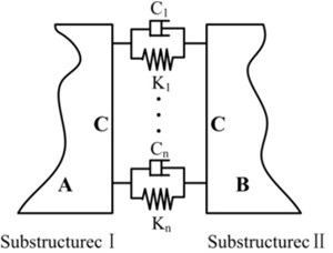
Two substructures represented as I and II are connected by the joints that are assumed as a combination of linear springs and dampers to form the assembly as shown in Fig. 1 [6, 18, 19, 20]. A and B represent the non-joint regions belonging to substructure I and II respectively, and C represents the joints regions. $K_{n}$ and $C_{n}$ mean the joints stiffness and damping values respectively. Joints properties identification is focused mainly on the determination of the stiffness and damping values.

2.1. Basic identification formulas

According to Fig. 1, the input-output relationship of the unconstrained substructures I and II can be expressed as:

1

M \ddot{X} + C \dot{X} + K X = F,

2

[\begin{array}{l} M_{n n} & M_{n c} \\ M_{c n} & M_{c c} \end{array}] \{\begin{array}{l} {\ddot{X}}_{n} \\ {\ddot{X}}_{c} \end{array}\} + [\begin{array}{l} C_{n n} & C_{n c} \\ C_{c n} & C_{c c} \end{array}] \{\begin{array}{l} {\dot{X}}_{n} \\ {\dot{X}}_{c} \end{array}\} + [\begin{array}{l} M_{n n} & M_{n c} \\ M_{c n} & M_{c c} \end{array}] \{\begin{array}{l} X_{n} \\ X_{c} \end{array}\} = \{\begin{array}{l} F_{n} \\ F_{c} \end{array}\},

where $M$ , $C$ and $K$ are the mass matrix, damping matrix and stiffness matrix not containing the properties of the joints. $X_{n}$ and $F_{n}$ represent the displacement and force vectors of the nodes relating to the non-joints regions respectively. $X_{c}$ and $F_{c}$ are the displacement and force vectors of the joints region nodes.

Thus the dynamic stiffness of the unconstrained substructures is:

3

Z = - ω^{2} [\begin{array}{l} M_{n n} & M_{n c} \\ M_{c n} & M_{c c} \end{array}] + j ω [\begin{array}{l} C_{n n} & C_{n c} \\ C_{c n} & C_{c c} \end{array}] + [\begin{array}{l} K_{n n} & K_{n c} \\ K_{c n} & K_{c c} \end{array}] = [\begin{array}{l} Z_{n n} & Z_{n c} \\ Z_{c n} & Z_{c c} \end{array}]

= {[H]}^{- 1} = {[\begin{array}{l} H_{n n} & H_{n c} \\ H_{c n} & H_{c c} \end{array}]}^{- 1},

where $H$ is the frequency response function matrix of the substructures.

The input-output relationship of the assembly can be written as:

4

M \ddot{X} + (C + C_{c}) \dot{X} + (K + K_{c}) X = F,

5

[\begin{array}{l} M_{n n} & M_{n c} \\ M_{c n} & M_{c c} \end{array}] \{\begin{array}{l} {\ddot{X}}_{n} \\ {\ddot{X}}_{c} \end{array}\} + [\begin{array}{l} C_{n n} & C_{n c} \\ C_{c n} & C_{c c} + C_{c} \end{array}] \{\begin{array}{l} {\dot{X}}_{n} \\ {\dot{X}}_{c} \end{array}\} + [{\begin{array}{l} K_{n n} & K_{n c} \\ K_{c n} & K_{c c} + K \end{array}}_{c}] \{\begin{array}{l} X_{n} \\ X_{c} \end{array}\} = \{\begin{array}{l} F_{n} \\ F_{c} \end{array}\},

where $C_{c}$ and $K_{c}$ are the damping and stiffness matrixes of the joints respectively.

Thus the dynamic stiffness of the constrained substructures is:

6

\tilde{Z} = - ω^{2} [\begin{array}{l} M_{n n} & M_{n c} \\ M_{c n} & M_{c c} \end{array}] + j ω [\begin{array}{l} C_{n n} & C_{n c} \\ C_{c n} & C_{c c} + C_{c} \end{array}] + [{\begin{array}{l} K_{n n} & K_{n c} \\ K_{c n} & K_{c c} + K \end{array}}_{c}]

= Z + [\begin{array}{l} 0 & 0 \\ 0 & K_{c} \end{array}] + j ω [\begin{array}{l} 0 & 0 \\ 0 & C_{c} \end{array}] = [\begin{array}{l} {\tilde{Z}}_{n n} & {\tilde{Z}}_{n c} \\ {\tilde{Z}}_{c n} & {\tilde{Z}}_{c c} \end{array}] = {[\tilde{H}]}^{- 1} = {[\begin{array}{l} {\tilde{H}}_{n n} & {\tilde{H}}_{n c} \\ {\tilde{H}}_{c n} & {\tilde{H}}_{c c} \end{array}]}^{- 1},

where $\tilde{H}$ is the frequency response function matrix of the assembly.

With Eqs. (3) and (6), the relationship between the dynamic stiffness of the substructures and the assembly are represented as:

7

\tilde{Z} - Z = {[\tilde{H}]}^{- 1} - {[H]}^{- 1} = [\begin{array}{l} 0 & 0 \\ 0 & K_{c} \end{array}] + j ω [\begin{array}{l} 0 & 0 \\ 0 & C_{c} \end{array}] = [\begin{array}{l} 0 & 0 \\ 0 & P \end{array}],

where $P = K_{c} + j ω C_{c}$ . $P$ includes the stiffness and damping values to be identified.

As excessive matrix inverse computations can affect the identification accuracy, Eq. (7) can be transformed to:

8

H - \tilde{H} = \tilde{H} [\begin{array}{l} 0 & 0 \\ 0 & P \end{array}] H .

The Eq. (8) can be expanded to:

9

[\begin{array}{l} H_{n n} - {\tilde{H}}_{n n} & H_{n c} - {\tilde{H}}_{n c} \\ H_{c n} - {\tilde{H}}_{c n} & H_{c c} - {\tilde{H}}_{c c} \end{array}] = [\begin{array}{l} {\tilde{H}}_{n c} P H_{c n} & {\tilde{H}}_{n c} P H_{c c} \\ {\tilde{H}}_{c c} P H_{c n} & {\tilde{H}}_{c c} P H_{c c} \end{array}] .

It is obvious that four basic formulas about FRFs of the substructures, the joints and the assembly can be extracted from Eq. (9):

10

H_{n n} - {\tilde{H}}_{n n} = {\tilde{H}}_{n c} P H_{c n},

11

H_{c c} - {\tilde{H}}_{c c} = {\tilde{H}}_{c c} P H_{c c},

12

H_{n c} - {\tilde{H}}_{n c} = {\tilde{H}}_{n c} P H_{c c},

13

H_{c n} - {\tilde{H}}_{c n} = {\tilde{H}}_{c c} P H_{c n} .

These basic formulas are for the identification of the joint dynamic properties. If $H_{n n}$ , ${\tilde{H}}_{n n}$ , $H_{c c}$ , ${\tilde{H}}_{c c}$ , $H_{n c}$ , ${\tilde{H}}_{n c}$ , $H_{c n}$ and ${\tilde{H}}_{c n}$ are accurately measured, every single formula of Eqs. (10)-(13) can be independently utilized to compute $P$ .

2.2. Identification of the stiffness constants and damping coefficients

Assume that there are $N$ pairs of springs and dampers to simulate the effectiveness of the joints. Thus there are 2 $N$ joint nodes. Adopting Eq. (11) to identify the joint parameters, then $H_{c c}$ , ${\tilde{H}}_{c c}$ and $P$ can be wrote as:

14

H_{c c} = [\begin{matrix} h_{11} & h_{12} & \dots & h_{12 n - 1} & h_{12 n} \\ h_{21} & h_{22} & \dots & h_{22 n - 1} & h_{22 n} \\ ⋮ & ⋮ & ⋮ & ⋮ \\ h_{2 n - 11} & h_{2 n - 12} & \dots & h_{2 n - 12 n - 1} & h_{2 n - 12 n} \\ h_{2 n 1} & h_{2 n 2} & \dots & h_{2 n 2 n - 1} & h_{2 n 2 n} \end{matrix}],

15

{\tilde{H}}_{c c} = [\begin{matrix} {\tilde{h}}_{11} & {\tilde{h}}_{12} & \dots & {\tilde{h}}_{12 n - 1} & {\tilde{h}}_{12 n} \\ {\tilde{h}}_{21} & {\tilde{h}}_{22} & \dots & {\tilde{h}}_{22 n - 1} & {\tilde{h}}_{22 n} \\ ⋮ & ⋮ & ⋮ & ⋮ \\ {\tilde{h}}_{2 n - 11} & {\tilde{h}}_{2 n - 12} & \dots & {\tilde{h}}_{2 n - 12 n - 1} & {\tilde{h}}_{2 n - 12 n} \\ {\tilde{h}}_{2 n 1} & {\tilde{h}}_{2 n 2} & \dots & {\tilde{h}}_{2 n 2 n - 1} & {\tilde{h}}_{2 n 2 n} \end{matrix}],

16

\begin{matrix} P = d i a g (\begin{array}{l} P_{1} & \dots & P_{i} & \dots & P_{n} \end{array}), \\ P_{i} = [\begin{matrix} k_{i} + j ω c_{i} & - k_{i} - j ω c_{i} \\ - k_{i} - j ω c_{i} & k_{i} + j ω c_{i} \end{matrix}], \end{matrix}

where $k_{i}$ and $c_{i}$ represent the stiffness and damping values of the $i$ th pair respectively.

Then Eq. (11) can be rewritten as:

17

[\begin{array}{l} H_{11} - {\tilde{H}}_{11} & H_{12} - {\tilde{H}}_{12} & \dots & H_{1 n} - {\tilde{H}}_{1 n} \\ H_{21} - {\tilde{H}}_{21} & H_{22} - {\tilde{H}}_{22} & \dots & H_{2 n} - {\tilde{H}}_{2 n} \\ ⋮ & ⋮ & ⋮ \\ H_{n 1} - {\tilde{H}}_{11} & H_{n 2} - {\tilde{H}}_{n 2} & \dots & H_{n n} - {\tilde{H}}_{n n} \end{array}]

= [\begin{array}{l} \sum {\tilde{H}}_{1 i} P_{i} H_{i 1} & \sum {\tilde{H}}_{1 i} P_{i} H_{i 2} & \dots & \sum {\tilde{H}}_{1 i} P_{i} H_{i n} \\ \sum {\tilde{H}}_{2 i} P_{i} H_{i 1} & \sum {\tilde{H}}_{2 i} P_{i} H_{i 2} & \dots & \sum {\tilde{H}}_{2 i} P_{i} H_{i n} \\ ⋮ & ⋮ & ⋮ \\ \sum {\tilde{H}}_{n i} P_{i} H_{i 1} & \sum {\tilde{H}}_{n i} P_{i} H_{i 2} & \dots & \sum {\tilde{H}}_{n i} P_{i} H_{i n} \end{array}],

where:

H_{n n} = [\begin{array}{l} h_{2 n - 12 n - 1} & h_{2 n - 12 n} \\ h_{2 n 2 n - 1} & h_{2 n 2 n} \end{array}], {\tilde{H}}_{n n} = [\begin{array}{l} {\tilde{h}}_{2 n - 12 n - 1} & {\tilde{h}}_{2 n - 12 n} \\ {\tilde{h}}_{2 n 2 n - 1} & {\tilde{h}}_{2 n 2 n} \end{array}] .

The element locates in the $m$ th row and $l$ th column of the right matrix belonging to Eq. (17) are expanded as:

18

\sum {\tilde{H}}_{m i} P_{i} H_{i l} = {\tilde{H}}_{m 1} P_{1} H {}_{1 l} + {\tilde{H}}_{m 2} P_{2} H {}_{2 l} + \dots + {\tilde{H}}_{m n} P_{n} H {}_{n l} .

For the direct FRFs having more reliability, let the diagonal elements of the left and right matrixes in Eq. (17) equal, thus a system of linear equations can be obtained to identify $P$ :

19

(\begin{matrix} h_{11} - {\tilde{h}}_{11} \\ h_{22} - {\tilde{h}}_{22} \\ ⋮ \\ h_{2 n - 12 n - 1} - {\tilde{h}}_{2 n - 12 n - 1} \\ h_{2 n 2 n} - {\tilde{h}}_{2 n 2 n} \end{matrix}) = (\begin{matrix} \sum ({\tilde{h}}_{12 i - 1} - {\tilde{h}}_{12 i}) (h_{12 i - 1} - h_{12 i}) {\hat{p}}_{i} \\ \sum ({\tilde{h}}_{22 i - 1} - {\tilde{h}}_{22 i}) (h_{22 i - 1} - h_{22 i}) {\hat{p}}_{i} \\ ⋮ \\ \sum ({\tilde{h}}_{2 n - 12 i - 1} - {\tilde{h}}_{2 n - 12 i}) (h_{2 n - 12 i - 1} - h_{2 n - 12 i}) {\hat{p}}_{i} \\ \sum ({\tilde{h}}_{2 n 2 i - 1} - {\tilde{h}}_{2 n 2 i}) (h_{2 n 2 i - 1} - h_{2 n 2 i}) {\hat{p}}_{i} \end{matrix})

= [\begin{matrix} ({\tilde{h}}_{11} - {\tilde{h}}_{12}) (h_{11} - h_{12}) & \dots & ({\tilde{h}}_{12 n - 1} - {\tilde{h}}_{12 n}) (h_{12 n - 1} - h_{12 n}) \\ ({\tilde{h}}_{21} - {\tilde{h}}_{21}) (h_{21} - h_{22}) & \dots & ({\tilde{h}}_{22 n - 1} - {\tilde{h}}_{22 n}) (h_{22 n - 1} - h_{22 n}) \\ ⋮ & ⋮ \\ ({\tilde{h}}_{2 n - 11} - {\tilde{h}}_{2 n - 12}) (h_{2 n - 11} - h_{2 n - 12}) & \dots & ({\tilde{h}}_{2 n - 12 n - 1} - {\tilde{h}}_{2 n - 12 n}) (h_{2 n - 12 n - 1} - h_{2 n - 12 n}) \\ ({\tilde{h}}_{2 n 1} - {\tilde{h}}_{2 n 2}) (h_{2 n 1} - h_{2 n 2}) & \dots & ({\tilde{h}}_{2 n 2 n - 1} - {\tilde{h}}_{2 n 2 n}) (h_{2 n 2 n - 1} - h_{2 n 2 n}) \end{matrix}] [\begin{matrix} {\hat{p}}_{1} \\ ⋮ \\ {\hat{p}}_{i} \\ ⋮ \\ {\hat{p}}_{n} \end{matrix}],

where ${\hat{p}}_{i} = k_{i} + j ω c_{i}$ . And Eq. (19) can be rewritten in a compact form as:

20

B = E \hat{P} .

Apparently, the formulas to identify joints parameters are in the complex domain. Thus $B$ , $E$ and $\hat{P}$ can be divided into a real and an imaginary parts respectively.

Then Eq. (20) can be rewritten as:

21

\{\begin{array}{l} B_{R} \\ B_{I} \end{array}\} = [\begin{array}{l} E_{R} & - ω E_{I} \\ E_{I} & ω E_{R} \end{array}] [\begin{array}{l} K \\ C \end{array}],

where $K$ and $C$ can be expressed as:

22

K = {[\begin{array}{l} k_{1} & k_{2} & \dots & k_{n} \end{array}]}^{T}, C = {[\begin{array}{l} c_{1} & c_{2} & \dots & c_{n} \end{array}]}^{T} .

As the real and the imaginary parts are apart, Eq. (20) is transformed into a system of real linear equations simplified as:

23

\tilde{B} = \tilde{E} [\begin{array}{l} K \\ C \end{array}] .

For different sampling frequencies, Eq. (23) can be expanded as:

24

\{\begin{array}{l} {\tilde{B}}_{ω 1} \\ {\tilde{B}}_{ω 2} \\ ⋮ \\ {\tilde{B}}_{ω m} \end{array}\} = \{\begin{array}{l} {\tilde{E}}_{ω 1} \\ {\tilde{E}}_{ω 2} \\ ⋮ \\ {\tilde{E}}_{ω m} \end{array}\} \{\begin{array}{l} K \\ C \end{array}\} .

And Eq. (24) can be simplified as:

25

\hat{B} = \hat{E} \{\begin{array}{l} K \\ C \end{array}\},

where $\hat{E}$ is a $4 m n \times 2 n$ matrix.

To solve the overdetermined Eq. (25), the least-square method is utilized to obtain the solution [6, 18, 21]. Thus Eq. (25) is transformed into Eq. (26) to identify the joint stiffness $K$ and damping values $C$ :

26

{\hat{E}}^{T} \hat{B} = {\hat{E}}^{T} \hat{E} \{\begin{array}{l} K \\ C \end{array}\},

where ${\hat{E}}^{T}$ is the transpose matrix of $\hat{E}$ .

2.3. The complete FRFs

As discussed in Section 1, the inaccessible FRFs in an experiment will make this identification method aforementioned almost impossible. As a consequence, many of the current identification methods have to use the incomplete data. In this paper, a method to estimate the unmeasured FRFs is developed.

As the FRFs of the unconstrained substructures can be obtained in an experiment, $H_{n n}$ , $H_{n c}$ , $H_{c n}$ and $H_{c c}$ can be measured directly. For the assembly, ${\tilde{H}}_{n n}$ can be measured directly, however, ${\tilde{H}}_{c c}$ and ${\tilde{H}}_{n c}$ (or ${\tilde{H}}_{c n}$ ) containing the joint nodes are inaccessible in the experiment.

Combining Eqs. (10) and (12) yields:

27

{\tilde{H}}_{n c} = H_{n c} - (H_{n n} - {\tilde{H}}_{n n}) H_{_{c n}}^{- 1} H_{c c} .

Combining Eqs. (11) and (13) yields:

28

{\tilde{H}}_{c c} = H_{c c} - (H_{c n} - {\tilde{H}}_{c n}) H_{_{c n}}^{- 1} H_{c c} .

By utilizing those measured FRFs, all the unmeasured FRFs can be estimated. With the complete FRFs, the bolt joints stiffness and damping values can be identified by using the algorithm proposed in Section 2.2.

3. Experimental case study

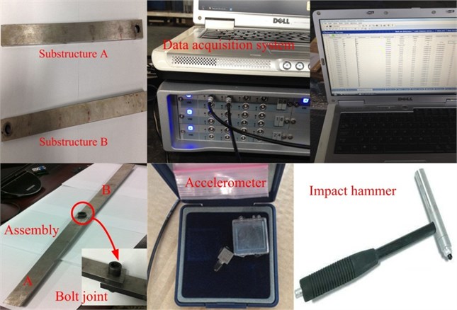
To validate the feasibility of the proposed identification method, vibration experiment was conducted. Two beams of dimensions 350×10×30 mm and 350×10×30 mm are defined as the substructures (Fig. 2 and Fig. 3). Their properties, including the materials, roughness and density, are listed in Table 1. Substructures A and B are the same. These two beams are assembled by one bolt M12 (Fig. 2 and Fig. 3). A torque of 10 N·m is applied on the screw.

Table 1Properties of the substructures

Substructures	Materials	Elastic modulus (GPa)	Density (kg/m³)	Poisson ratio	Roughness
A	Steel	206	7800	0.3	1.6
B	Steel	206	7800	0.3	1.6

Fig. 2The attachments used in the vibration experiment

3.1. Experimental scheme

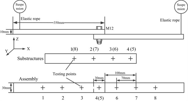
The experiment mainly dedicates to identifying the normal properties of the bolt joints. Distribution of the points to exert the excitations and pick up the responses is arranged as Fig. 3 shown. Four testing points are distributed along each single substructure. Totally eight testing points are determined in an assembly, and their locations are the same with those at the corresponding substructures. Points 4 and 5 are in the joint region, which are difficult to be measured for an assembly. In order to simulate the free-free boundary, the substructures and the assembly are suspended by two elastic ropes. Positions to hang them are determined by their calculated node points of their first bending eigenmodes.

Fig. 3Arrangement of the vibration experiment

3.2. The vibration experimental

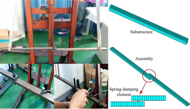
The experiment is shown in Fig. 4. The frequency range is focused on 0-3200 Hz and 1025 sampling frequencies are determined. In the experiment, the impulse hammer is moved to conduct the excitation at these testing points. The exciting force is in $Z$ direction. Two accelerometers are adopted to pick up the normal and tangential responses. Parameters related to the measurement equipment are list in Table 2.

Fig. 4The vibration experiment and the simulation

The substructures are measured at first and later the assembly. Movements of the impulse hammer and the accelerometers are in order according to the assigned number in Fig. 4 to ensure that all FRFs of each single testing point are measured. To obtain the experimental information of the assembly at the inaccessible points 4 and 5, the impulse hammer and accelerometers should be placed near them as close as possible. However, these measured FRFs of points 4 and 5 are not used in the identification, and they are only utilized to validate the accuracy of the estimated FRFs.

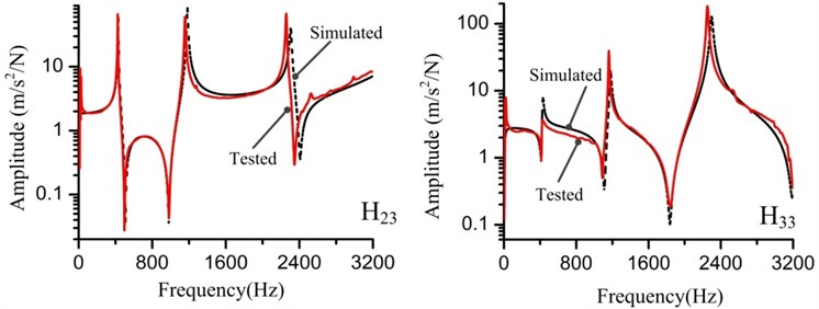
To calibrate the FEM of the substructures, modal parameters and FRFs of the measured and the simulated are compared. FRFs defined as $H_{23}$ and $H_{33}$ are depicted in Fig. 5, in which the measured and simulated FRFs are in good agreement. The modal parameters are listed in Table 3, and the damping ratio error of the 3rd mode is relatively high. After analyzing the mode shape of the 3rd mode, we find that the substructure sways in the $X Y$ plane. As the force was exerted only in $Z$ direction and one accelerometer pasted in the $Y$ direction, the direct FRFs in $Y$ direction could not be achieved, and it causes the tangential information to have a worse reliability. However, the synthetized comparison results mean that we can use the FEMs of the substructures to compose the FEM of the assembly.

Table 2Parameters related the measurement equipment

Name	Type	Sensibility	Weight
Impulse hammer	PCB 086D05	0.23 mV/N	0.32 Kg
Accelerometer Y	ICP	99.8 mv/g	4 g
Accelerometer Z	ICP	100.3 mv/g	4 g

Table 3Tested and simulated modal properties of the substructures

Mode number	Natural frequency (Hz)		Damping ratios		Error (%)
Mode number	Measured	Simulated	Measured	Simulated	Frequency	Damping ratios
1st	420.2	430.27	1.25 %	1.25 %	2.4 %	0
2nd	1158.8	1181.9	0.52 %	0.53 %	1.99 %	1.9 %
3rd	1271.9	1263.3	0.41 %	0.51 %	0.67 %	24.4 %
4th	2251.1	2305.3	0.39 %	0.39 %	2.4 %	0

Fig. 5FRFs (H23 and H33) of the experiment and finite element analysis for the substructures

4. Estimation of the unmeasured FRFs

To obtain the complete FRFs, the measured partial information is used to estimate the inaccessible FRFs of the points 4 and 5. The computations based on Eqs. (27) and (28) are expressed as:

29

[\begin{array}{l} {\tilde{h}}_{14} & {\tilde{h}}_{15} \\ {\tilde{h}}_{24} & {\tilde{h}}_{25} \\ {\tilde{h}}_{34} & {\tilde{h}}_{35} \\ {\tilde{h}}_{64} & {\tilde{h}}_{65} \\ {\tilde{h}}_{74} & {\tilde{h}}_{75} \\ {\tilde{h}}_{84} & {\tilde{h}}_{85} \end{array}] = [\begin{array}{l} h_{14} & h_{15} \\ h_{24} & h_{25} \\ h_{34} & h_{35} \\ h_{64} & h_{65} \\ h_{74} & h_{75} \\ h_{84} & h_{85} \end{array}] - ([\begin{array}{l} h_{11} & h_{12} & h_{13} & h_{16} & h_{17} & h_{18} \\ h_{21} & h_{22} & h_{23} & h_{26} & h_{27} & h_{28} \\ h_{31} & h_{32} & h_{33} & h_{36} & h_{37} & h_{38} \\ h_{61} & h_{63} & h_{63} & h_{66} & h_{67} & h_{68} \\ h_{71} & h_{72} & h_{73} & h_{76} & h_{77} & h_{78} \\ h_{81} & h_{82} & h_{83} & h_{86} & h_{87} & h_{88} \end{array}] - [\begin{array}{l} {\tilde{h}}_{11} & {\tilde{h}}_{12} & {\tilde{h}}_{13} & {\tilde{h}}_{16} & {\tilde{h}}_{17} & {\tilde{h}}_{18} \\ {\tilde{h}}_{21} & {\tilde{h}}_{22} & {\tilde{h}}_{23} & {\tilde{h}}_{26} & {\tilde{h}}_{27} & {\tilde{h}}_{28} \\ {\tilde{h}}_{31} & {\tilde{h}}_{32} & {\tilde{h}}_{33} & {\tilde{h}}_{36} & {\tilde{h}}_{37} & {\tilde{h}}_{38} \\ {\tilde{h}}_{61} & {\tilde{h}}_{63} & {\tilde{h}}_{63} & {\tilde{h}}_{66} & {\tilde{h}}_{67} & {\tilde{h}}_{68} \\ {\tilde{h}}_{71} & {\tilde{h}}_{72} & {\tilde{h}}_{73} & {\tilde{h}}_{76} & {\tilde{h}}_{77} & {\tilde{h}}_{78} \\ {\tilde{h}}_{81} & {\tilde{h}}_{82} & {\tilde{h}}_{83} & {\tilde{h}}_{86} & {\tilde{h}}_{87} & {\tilde{h}}_{88} \end{array}])

\cdot {[\begin{array}{l} h_{41} & h_{42} & h_{43} & h_{46} & h_{47} & h_{48} \\ h_{51} & h_{52} & h_{53} & h_{56} & h_{57} & h_{58} \end{array}]}^{- 1} \cdot [\begin{array}{l} h_{44} & h_{45} \\ h_{54} & h_{55} \end{array}],

30

[\begin{array}{l} {\tilde{h}}_{44} & {\tilde{h}}_{45} \\ {\tilde{h}}_{54} & {\tilde{h}}_{55} \end{array}] = [\begin{array}{l} h_{44} & h_{45} \\ h_{54} & h_{55} \end{array}] - ([\begin{array}{l} h_{41} & h_{42} & h_{43} & h_{46} & h_{47} & h_{48} \\ h_{51} & h_{52} & h_{53} & h_{56} & h_{57} & h_{58} \end{array}] - [\begin{array}{l} {\tilde{h}}_{41} & {\tilde{h}}_{42} & {\tilde{h}}_{43} & {\tilde{h}}_{46} & {\tilde{h}}_{47} & {\tilde{h}}_{48} \\ {\tilde{h}}_{51} & {\tilde{h}}_{52} & {\tilde{h}}_{53} & {\tilde{h}}_{56} & {\tilde{h}}_{57} & {\tilde{h}}_{58} \end{array}])

∙ {[\begin{array}{l} h_{41} & h_{42} & h_{43} & h_{46} & h_{47} & h_{48} \\ h_{51} & h_{52} & h_{53} & h_{56} & h_{57} & h_{58} \end{array}]}^{- 1} \cdot [\begin{array}{l} h_{44} & h_{45} \\ h_{54} & h_{55} \end{array}] .

The estimated and tested FRFs ${\tilde{H}}_{14}$ and ${\tilde{H}}_{34}$ are depicted in Fig. 6, and the estimated results are consistent well with the tested results.

5. Identification of the joints stiffness and damping

As the complete FRFs have been obtained, the blot joints stiffness and damping values can be identified based on the algorithm mentioned in Section 2.2. The identified stiffness constant and damping values are 7.8×10⁷ N/m and 2741 N·s/m respectively.

Fig. 6Measured and estimated FRFs (H~14 and H~34) of the assembly for the substructures

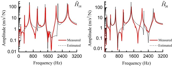
Fig. 7Measured and simulated FRFs (H~44) of the assembly for the substructures

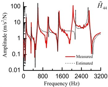
Table 4Tested and simulated modal properties of the assembly

Mode number	Natural frequency (Hz)		Damping ratios		Error (%)
Mode number	Measured	Simulated	Measured	Simulated	Frequency	Damping ratios
1st	318.9	323.6	0.57 %	0.59 %	1.5 %	3.5 %
2nd	438.5	430.3	0.21 %	0.23 %	1.9 %	9.5 %
3rd	1018.1	1039.5	0.14 %	0.13 %	2.1 %	7.4 %
4th	1163.1	1181.9	0.10 %	0.11 %	1.5 %	10 %
5th	1763.6	1769.3	0.26 %	0.24 %	0.3 %	7.7 %
6th	2052.3	2144.9	0.18 %	0.18 %	4.5 %	0
7th	2715.1	2721.2	0.16 %	0.15 %	0.2 %	6.3%

In the FEM of the assembly, the two substructures are connected by the spring-damping element (shown in Fig. 4). The identified parameters are applied to the spring-damping element. Utilizing the assembled FEM to conduct a modal analysis and a harmonic analysis, the simulated and tested modal properties are listed in Table 4 and FRFs ( ${\tilde{H}}_{44}$ ) are shown in Fig. 7. The errors of the modal parameters are relatively low and the curves of the measured and simulated FRFs coincide with each other very well. These comparisons validate the accuracy of the identification method mentioned in Section 2.

6. Application in a machine tool

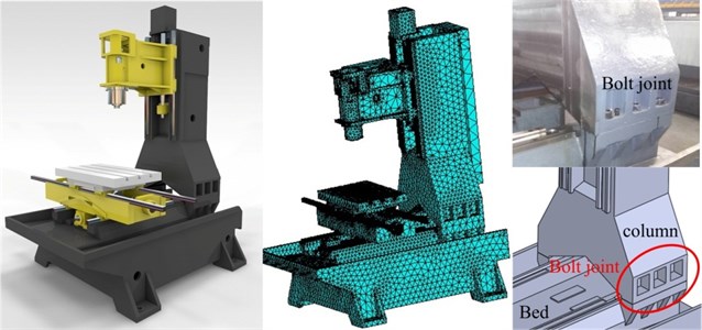
Machine tool is an integrated assembly composed by many basic components, such as the bed, the column, the headstock and so on. The continuity of the machine tool is destroyed by the existence of the joints. Bolt joint as one conventional joint in a machine tool, its properties have great effects on the dynamic characteristics of the whole machine tool. To build the accurate FEM of the whole machine tool, it is important to simulate the bolt joints properties. Adopting the spring-damping elements to simulate the bolt joints in the FEM of the whole machine tool, the proposed identification method in this paper is applied in the machine tool to identify the stiffness and damping values.

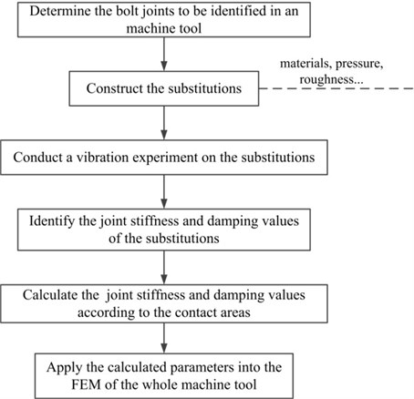
As researches have discussed that if the average contact pressure of the joints are the same, their dynamic characteristics parameters of the unite area are the same [16, 17, 22]. Thus, the joints to be identified in a machine tool can be analyzed using the substitutions with the same contact conditions (pressure, materials and roughness). Using the substitutions to conduct the vibration experiment to obtain the FRFs, the joints stiffness and damping values are identified based on the approaches mentioned in Section 2 and 3. The stiffness and damping values of the bolt joints in a machine tool can be calculated according to the contact area relationship between them and the substitutions. Then the calculated parameters can be applied to in the FEM of the whole machine tool.

The application was implemented in a vertical machining center (shown in Fig. 9) according to the flowchart shown in Fig. 8.

Fig. 8The flowchart to realize the application

In the vertical machining center, the bed-column bolt joint is mainly focused on. The bed and column are connected by six bolts M20 and a torque of 500 N·m is applied on each screw. Properties of the bed-column joint are listed in Table 5. By consulting Ref. [23], the calculated pressure of the joints is 13.56 MPa.

Table 5Properties of the bed-column joint

Substructures	Materials	Elastic modulus (GPa)	Density (kg/m³)	Poisson ratio	Roughness
A	HT250	130	7300	0.25	1.6
B	HT250	130	7300	0.25	1.6

Fig. 9The studied whole vertical machining center

The assembled free-free beams with a bolt joint is constructed according to the bed-column joint. Its dimensional parameters are the same with the beams in Section 3. To equal the pressure, the calculated torque to be applied on the screw is 22.5 N·m.

The vibration experiment was conducted according to the arrangements mentioned in Section 3.3. With the tested FRFs, the inaccessible FRFs were estimated. And the calculated stiffness and damping values are 4.9×10¹⁰ and 1.1×10⁶ N·s/m

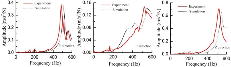
Applying the identified parameters in the FEM of the whole vertical machining center, its top ten natural frequencies and FRFs at the spindle tip are listed in Table 6 (marked as simulated I) and depicted in Fig. 11 respectively.

To validate the accuracy of the whole vertical machining center FEM, vibration experiment about the whole machine tool were executed. The experiment is shown in Fig. 10. The external exciting force was exerted by the impact hammer and the hammer was moved to exert the exciting force at different parts of the whole vertical machining center. The hammering positions were arranged to avoid at the nodal points predicted by the finite element modal analysis. Three accelerometers were pasted at the spindle nose marked as $X$ , $Y$ and $Z$ to obtain the response signals in three directions as shown in Fig. 10. The force and accelerance signals were recorded by the LMS vibration testing system, and they were processed to obtain the FRFs. When hammering at the positions marked as $X$ , $Y$ and $Z$ to get the direct FRFs, the hammer was as close as possible to these acceleration sensors. Taking the working conditions of the machine tool into consideration, the dynamic characteristics between 0-600 Hz was mainly focused on. The tested natural frequencies and FRFs curves are listed in Table 6 (marked as tested) and depicted in Fig. 11 respectively. The accordance of the measured and simulated results demonstrates that the whole vertical machining center FEM based on the joints characteristics is accurate.

To study on how the bed-column joint characteristics affect the dynamics of the whole machine tool, another FEM in which the bed and the column were bonded together was established to obtain the natural frequencies. The simulated results are also listed in Table 6 (marked as simulated II). The natural frequencies differ from the tested and the previously simulated results obviously, which further stress the importance to take the joints characteristics into consideration when constructing an accurate whole machine tool FEM to analyze its dynamic characteristics.

Table 6Natural frequency of the whole machine tool

	Natural frequency (Hz)
Mode number	1	2	3	4	5	6	7	8	9	10
Tested	50.2	81.9	118.7	131.2	143.5	158.9	169.3	188.3	213.1	251.0
Simulated I	50.1	75.0	114.2	137.5	143.6	151.5	162.1	180.2	205.6	257.3
Simulated II	58.7	94.6	131.6	148.2	171.6	189.1	204.8	226.7	272.3	300.5
Error I (%)	0.2	8.5	3.8	4.8	0.07	4.7	4.3	4.3	3.5	2.5
Error II (%)	16.9	15.4	10.9	13.0	19.6	19	20.1	20.4	27.8	19.7

Fig. 10The experiment conducted on the whole machine tool

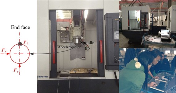
Fig. 11The FRFs in three directions at the spindle tip

7. Conclusions

A general method to identify the bolt joints dynamic parameters is proposed in this paper, and it has been applied in machine tools. This method provides an easy way to extract the dynamic stiffness constants and damping values of a single bolt joint by estimating the unmeasured FRFs and avoiding inverse calculation to the frequency response function matrix directly. An experiment on assembled free-free steel beams with a bolt joint to verify this method has been demonstrated. Experiment on the whole vertical machining center validates the successful application of the identification method in machine tools. Some important conclusions are as follows.

1) As the main application of this identification method is in machine tools, in which the nonlinearity behaviors of the bolt joints are suppressed, for they are tightly fastened. Only a combination of linear springs and dampers are adopted to simulate the joints properties. Basic algorithms to estimate the inaccessible FRFs with the partially measured information and identify the joints dynamic parameters with the complete FRFs are derived based on the substructuring method. Accuracy of the identification method is validated by the accordance of the tested and the simulated FRFs.

2) An approach is provided to identify the bolt joints parameters in a machine tool, and the identification of the bed-column bolt joint in a vertical machining center has described the application procedure. The obtained stiffness and damping values were used in the FEM of the whole machine tool to have the modal and harmonic analyses. The good agreement of the tested and the simulated natural frequencies and FRFs at the spindle tip demonstrates the successful application.

3) Modal parameters are compared between machine tool FEMs with the glued bed-column interfaces and the spring-damping elements simulated bed-column interfaces. The obvious differences demonstrate the importance to establish the accurate FEM of the whole machine tool by taking the joints parameters into account when well analyzing and predicting its dynamic behaviors.

References

Liang Y. C., Chen W. Q., Bai Q. S., Sun Y. Z., Chen G. D., Zhang Q., Sun Y. Design and dynamic optimization of an ultraprecision diamond flycutting machine tool for large KDP crystal machining. The International Journal of Advanced Manufacturing Technology, Vol. 69, 2013, p. 237-244.

Search CrossRef
Lee S. W., Mayor R., Ni J. Dynamic analysis of a mesoscale machine tool. Journal of Manufacturing Science and Engineering, Vol. 128, Issue 1, 2005, p. 194-203.

Search CrossRef
Zhang G. P., Huang Y. M., Shi W. H., Fu W. P. Predicting dynamic behaviors of a whole machine tool structure based on computer-aided engineering. International Journal of Machine Tools and Manufacture, Vol. 43, 2003, p. 699-706.

Search CrossRef
Okubo N., Miyazaki M. Development of uncoupling technique and its application. Proceedings of International Modal Analysis Conference, Florida, USA, 1984, p. 1194-1200.

Search CrossRef
Tsai J. S., Chou Y. F. The identification of dynamics characteristics of a single bolt joint. Journal of Sound and Vibration, Vol. 125, Issue 3, 1988, p. 487-502.

Search CrossRef
Wang J. H., Liou C. M. Identification of parameters of structural joints by use of noise-contaminated FRFs. Journal of Sound and Vibration, Vol. 142, Issue 2, 1990, p. 261-277.

Search CrossRef
Ren Y., Beards C. F. Identification of joint properties of a structure using FRF data. Journal of Sound and Vibration, Vol. 186, 1995, p. 567-587.

Search CrossRef
Ahmadian H., Jalali H. Identification of bolted lap joints parameters in assembled structures. Mechanical Systems and Signal Processing, Vol. 27, 2007, p. 1041-1050.

Search CrossRef
Lee D. H., Hwang W. S. An identification method for joint structural parameters using an FRF-based substructuring method and an optimization technique. Journal of Mechanical Science and Technology, Vol. 21, 2007, p. 2011-2022.

Search CrossRef
Yang T. C, Fan S. H., Lin C. S. Joint stiffness identification using FRF measurements. Computers and Structures, Vol. 81, 2003, p. 2549-2556.

Search CrossRef
Celic D., Boltezar M. Identification of the dynamic properties of joints using frequency-response functions. Journal of Sound and Vibration, Vol. 317, Issue 1-2, 2008, p. 158-174.

Search CrossRef
Wang M., Wang D., Zheng G. T. Joint dynamic properties identification with partially measured frequency response function. Mechanical Systems and Signal Processing, Vol. 27, 2012, p. 499-512.

Search CrossRef
Tol Ş., Ozguven H. N. Dynamic characterization of bolted joints using FRF decoupling and optimization. Mechanical Systems and Signal Processing, Vol. 54-55, 2015, p. 124-138.

Search CrossRef
Tian H. L., Li B., Liu H. Q., Mao K. M., Peng F. Y., Huang X. L. A new method of virtual material hypothesis-based dynamic modeling on fixed joint interface in machine tools. International Journal of Machine Tools and Manufacture, Vol. 51, Issue 3, 2011, p. 239-249.

Search CrossRef
Li W. L. A new method for structural model updating and joint stiffness identification. Mechanical Systems and Signal Processing, Vol. 16, Issue 1, 2002, p. 155-167.

Search CrossRef
Yoshihara M. Computer-aided design improvement of machine tool states incorporating joint dynamics data. Annals of the CIRP, Vol. 28, 1979, p. 241-246.

Search CrossRef
Yoshihara M. Measurement of dynamic rigidity and damping property for simplified joint models and simulation computer. Annals of the CIRP, Vol. 25, 1977, p. 193-198.

Search CrossRef
Guo T. N., Li L., Cai L. G., Liu Z. F., Zhao Y. S., Yang K. Identifying mechanical joint dynamic parameters based on measured frequency response functions. Journal of Vibration and Shock, Vol. 30, Issue 5, 2011, p. 69-72, (in Chinese).

Search CrossRef
Hwang H. Y. Identification techniques of structure connection parameters using frequency response functions. Journal of Sound and Vibration, Vol. 212, Issue 3, 1998, p. 469-479.

Search CrossRef
Mehrpouya M., Graham E., Park S. S. FRF based joint dynamics modeling and identification. Mechanical Systems and Signal Processing, Vol. 39, Issue 1-2, 2013, p. 265-279.

Search CrossRef
Celic D., Boltezar M. The influence of the coordinate reduction on the identification of the joint dynamic properties. Mechanical Systems and Signal Processing, Vol. 39, 2009, p. 1260-1271.

Search CrossRef
Mi L., Yin G. F., Sun M. N. Effects of preloads on joints on dynamic stiffness of a whole machine tool structure. Journal of Mechanical Science and Technology, Vol. 26, 2012, p. 495-508.

Search CrossRef
Deng C. Y, Yin G. F., Fang H., Meng Z. Y. X. Dynamic characteristics optimization for a whole vertical machining center based on the configuration of joint stiffness. The International Journal of Advanced Manufacturing Technology, Vol. 76, Issues 5-8, 2015, p. 1225-1242.

Search CrossRef

About this article

Received

19 January 2015

Accepted

11 April 2015

Published

15 May 2015

SUBJECTS

Mechanical vibrations and applications

Keywords

bolt joints identification

partially measured frequency response functions

machine tools

substructuring method

Acknowledgements

This research is sponsored by National Major Projects of High-End CNC Machine Tools and Basic Manufacturing Equipment (No. 2013ZX04005-012) and Science and Technology Support Project of Sichuan Province (No. 2014GZ0119).

This is an open access article distributed under the Creative Commons Attribution License, which permits unrestricted use, distribution, and reproduction in any medium, provided the original work is properly cited.