Abstract
In this paper, the QSSE method has been used for experimental study on parameter identification of rubber-bearings, the experimental model of rubber-bearings has been built and the widely used Bouc-Wen model has been investigated to represent the hysteretic behavior of rubber-bearing isolators. Further, experimental tests using a particular type of rubber-bearing (GZN110) have been conducted to measure base accelerations and model accelerations. Based on experimental vibration data measured from sensors, the QSSE method is used to identify the model parameters and displacements. Experimental results demonstrate that the estimated parameters are identical, and the identified displacements match the experimental ones well based on different excitation scenarios, i.e., different kinds of earthquakes with different peak ground accelerations. The influence on the estimated parameters based on the changes of initial parameters is little. It demonstrates that the Bouc-Wen model is capable of describing the nonlinear behavior of rubber-bearings. Compared with the EKF method, the QSSE method calculates faster, which demonstrates that the QSSE approach has better robustness and calculation efficiency and is quite effective and accurate for parameter identification of nonlinear hysteretic rubber-bearings.
1. Introduction
Earthquake is a random natural disaster which leads huge losses of people’s life property and economic construction. How to ensure the security of structure is a difficult problem of the civil structural health monitoring system that should be solved in modern buildings. In seismic passive control theory, the base isolation technology is a reasonable, effective, safe and economical method which can reduce or even avoid the structural damage from earthquake effectively[1].Nowadays the isolation technology is used more and more widely all over the world, and high damping rubber-bearings system has already been applied to buildings and bridges. In view of its significant decrease of the structural responses which are suffering earthquake or other dynamic loads, the base isolation system will be applied more and more widely.
Parameter identification is another important work of the civil structural health monitoring system. Recently, analysis methodologies for structural damage identification, based on measured vibration data, have been studied [4, 5]. In the literatures time domain approaches have been studied and developed. These include the least-squares estimation (LSE) [6, 7], the Bayesian state estimation method [8], the extended Kalman filter (EKF) [9-11], the H-infinite filter [12], the Monte Carlo filter [13] and the model-reference method [14], etc. In these methods, the LSE method and EKF method are used more widely. However, in the LSE approach, the applied displacement response is obtained through double numerical integrations and result in a significant drift that is also magnified by the structural damage. While the numerical drift can be corrected, it is difficult to accomplish online. In the EKF method, both the state vector and the parametric vector are estimated simultaneously. Since the dimension of the sum vectors if large, the computational effort required is quite involved. What’s worse, if the model is so complex, it is also difficult to accomplish online.
The literature [15] proposed a new approach, referred to as the quadratic sum-squares error (QSSE) approach, for the online or almost online system identification and damage detection of structures. One advantage of this method is that the unknown parametric vector is estimated directly first and the state vector is updated using estimated , thus reducing the computational efforts significantly and improving the calculation efficiency which is helpful for identification online. Meanwhile, this method has low limit upon initial values that can give a good result without an approximate initial value.
In this paper, the parameter identification experiment upon the rubber bearings was conducted to verify the availability, accuracy and stability of the QSSE approach. Firstly, the nonlinear and hysteretic model was built depending on the Bouc-Wen model which was widely used on nonlinear model building and some hysteretic parameters were set so as to simplify the model. Then the experimental structure, consisted of a mass block which was supported by eight rubber bearings, was excited upon earthquake wave. Finally, the model parameters were identified by the QSSE approach using the measured excitation signal and acceleration responses. The experimental results show that, the identified parameters upon the QSSE method are consistent due to different earthquake wave excitations with different peak values. The identified displacements and the measured displacements fit very well, thus proves that the QSSE method can identify the nonlinear hysteresis parameters effectively. Meanwhile, the change of initial values has little influence on the parameter identification in QSSE method. It proves that the QSSE method has a good robustness and the QSSE method can meet the needs of practical engineering application. What’s more, the operational times of the QSSE method are obviously less than that of EKF method in the same condition. It means that the QSSE method has better identification efficiency, and it can be applied online on practical engineering application easier that it has better practical value.
2. QSSE approach
Consider a m-DOF nonlinear structure:
In which -displacement vector, mass matrix, -damping force vector, -stiffness force vector, -excitation vector, and excitation influence matrix associated with . In Eq. (1), -unknown parametric vector with being the th unknown parameter of the structure, including damping, stiffness, nonlinear, and hysteretic parameters. For simplicity of derivation, we shall assume for the time being that the unknown parametric vector is constant, i.e., , where , and sampling time.
Introduce a state vector with a dimension of , i.e.:
One can transform the equation of motion in Eq. (1) into a state equation, i.e.:
In which model noise (uncertainty) vector with zero mean and a covariance matrix .
A nonlinear discrete equation for an observation vector (measured response) can be expressed as follows:
In which -dimensional observation vector, and measured s-dimensional excitation vector at , is an implicit function of the unknown parametric vector , and is a measurement noise vector assumed to be a Gaussian white noise vector with zero mean and a covariance matrix , where Kroneker delta. Our approach is to determine , by minimizing the sum-squares error between the measured data and their theoretical expressions .
The weighted sum-squares error (up to ) between the observation data and the analytical expression h in Eq. (4) is given by:
Let be the estimate of at and be the estimate of based on the estimated parametric vector . Since is a nonlinear function of the unknown vector , it will be linearized around the estimate of at the previous step , i.e., and as follows:
where:
In Eq. (10), is referred to as the sensitivity matrix of the state vector with respect to the parametric vector , i.e.:
and can be computed from as follows:
Substituting Eq. (6) into Eq. (5) with , one obtains the objective function , which is a quadratic function of unknown parametric vector , as follows:
in which:
Minimizing the quadratic objective function in Eq. (14) with respect to , we obtain the estimation for at in the following:
Similarly, the estimate for at is obtained as follows:
To derive the recursive solution for , i.e., the solution expressed in terms of , we make the following partitions:
The recursive solution for can be obtained by substituting Eq. (20-22) into Eq. (18) and using Eq. (19) with the result:
in which gain matrix and:
To start the recursive solution above, the initial values at , including , , , and should be assigned. The analytical solution derived in Eq. (23)-(26) is referred to as the QSSE approach.
In the derivation above, the state vector is first computed from Eq. (24) once is evaluated. The state vector is then updated by applying the Kalman filter with being estimated from Eq. (23), i.e.:
in which Kalman gain matrix:
and is given by:
3. Rubber bearings hysteretic model
The parameter identification experiment upon the rubber bearings was conducted to verify the availability of the QSSE approach. The nonlinear and hysteretic model was built depending on the Bouc-Wen model which was widely used on nonlinear model building. Under the base acceleration excitation , the motion equation of rubber-bearing system can be expressed as follows:
In which is inter-story drift, is hysteresis displacement component, and , , are system mass, damping and stiffness respectively. The hysteresis displacement component can be expressed by differential equation as follows:
So we can see that there are four hysteresis parameters , , , and two structure parameters and in the Bouc-Wen model. Usually can be 1 and then the parameters of the rubber-bearing hysteretic model will be reduced to be , , , and . And the parameters of natural rubber-bearing can use the reference values as follows: 0.5, 0.5, 2. Therefore the estimated parameter in this paper is .
4. Experimental studies
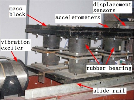
The rubber bearing used in this study was GZNΦ110 natural rubber bearing. The experimental model, as shown in Fig. 1, was a structure that one mass block which weight 115 kg supported by the rubber bearing. Firstly, the accelerometers PCB 3701G3FA3G and displacement sensors ASM WS10-250-10V-L10 were installed on the base and the upper mass block, then the vibration exciter and slide rail shaking table were used to simulate the base excitation, and at the same time the accelerometer and displacement singles were collected by the Q8 control board which produced by Canada Quanser company. In which the displacement responses were used to verify the effectiveness of the model and the feasibility and the accuracy of the QSSE method’s application in the parameter identification of the rubber bearing. The sampling frequency of all singles in the experiment is 500 Hz.
Fig. 1Experimental set-up
5. Validity analysis
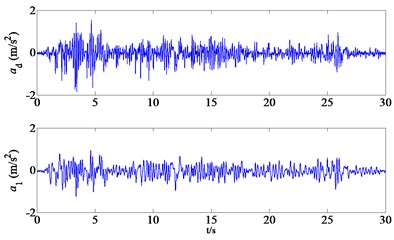
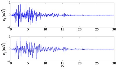
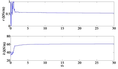
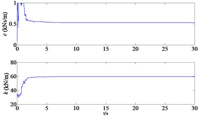
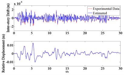
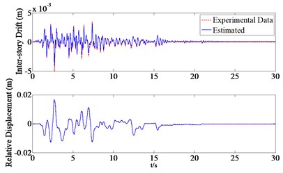
In the experiment, the N-S direction earthquake wave used El Centro and Kobe seismic wave accelerometer single separately, and the peak value were PGA = 0.2 g, PGA = 0.3 g, PGA = 0.4 g and PGA = 0.5 g respectively. Through measuring base accelerometer single and structure accelerometer response , the model unknown parameters – stiffness and damping were identified on-line by QSSE method. In which the initial values of the undetermined parameters are and . Take the case of PGA = 0.2 g as example, the base accelerometer single and structure accelerometer response were measured as shown in Fig. 2. The identified model parameters are shown as Fig. 3 depending on the measured accelerometers in Fig. 2 and the QSSE method. At the same time, the identified inter-story drifts and relative displacements are shown in Fig. 4, where the identified displacements indicated by a solid line while the measured displacements shown by a dotted line.
Compare the identified results depending on the above four cases, as shown in Table 1, we can see that the identified parameter values using QSSE method are consistent due to different earthquake wave excitations with different peak values.
Meanwhile, we can also see from the identified displacement results, as shown in Fig. 4, that the identified displacements and the measured displacements fit very well, thus proves that the QSSE method can identify the nonlinear hysteresis parameters effectively.
Fig. 2The excitation and acceleration output due to earthquake (PGA = 0.2 g): a) the excitation and acceleration output due to El Centro earthquake (PGA = 0.2 g), b) the excitation and acceleration output due to Kobe earthquake (PGA = 0.2 g)
a)
b)
Fig. 3The identified results of rubber bearing parameters due to earthquakes (PGA = 0.2 g): a) the identified parameters due to El Centro earthquake, b) the identified parameters due to Kobe earthquake
a)
b)
Fig. 4The identified results of rubber bearing relative displacements and inter-storey drifts due to earthquakes (PGA = 0.2 g): a) the identified displacements due to El Centro earthquake, b) the identified displacements due to Kobe earthquake
a)
b)
Table 1The identified results of structural parameters
PGA | Seismic wave | /(kN/m) | /(kNs/m) |
PGA = 0.2 g | El Centro | 60.89 | 0.53 |
Kobe | 59.54 | 0.53 | |
PGA = 0.3 g | El Centro | 61.02 | 0.54 |
Kobe | 59.43 | 0.54 | |
PGA = 0.4 g | El Centro | 61.39 | 0.53 |
Kobe | 59.10 | 0.52 | |
PGA = 0.5 g | El Centro | 60.50 | 0.52 |
Kobe | 58.82 | 0.52 |
6. Robustness analysis
In order to verify the robustness of QSSE method, the El Centro seismic wave with PGA = 0.2 g was imposed on the model with different initial values of damping and stiffness. Depending on the measured accelerometers and QSSE method, we get the identified results as shown in Table 2.
From Table 2, the identified parameters are almost the same with different initial values, which means that the change of initial values have little influence on the parameter identification in QSSE method. It proves that the QSSE method has a good robustness and the QSSE method can meet the needs of practical engineering application.
Table 2The identified results of structural parameters
Initial values | Identified values | ||
/(kN/m) | /(kNs/m) | /(kN/m) | /(kNs/m) |
30 | 0.1 | 60.89 | 0.53 |
40 | 0.1 | 60.86 | 0.53 |
40 | 0.2 | 60.88 | 0.53 |
40 | 0.5 | 60.89 | 0.52 |
50 | 0.2 | 60.90 | 0.52 |
70 | 0.5 | 60.92 | 0.52 |
7. Efficiency analysis
To verify the identification efficiency of QSSE method, this paper compared the QSSE method with classical EKF method on identification results of El Centro earthquake wave in which PGA = 0.2 g. The results of EKF method are shown in Fig. 5, and all operational times of two methods are shown in Table 3 with 5 times.
Fig. 5The identified parameters due to EKF method
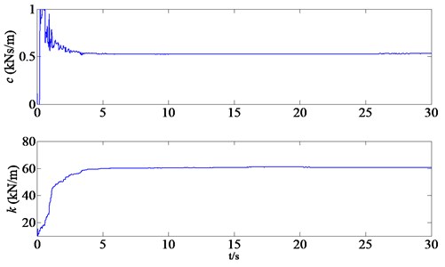
Table 3The operational times of two methods
QSSE time (s) | Average time (s) | EKF time (s) | Average time (s) |
1.2747 | 1.2546 | 4.0749 | 4.0929 |
1.2496 | 4.1971 | ||
1.2503 | 4.1054 | ||
1.2498 | 4.0336 | ||
1.2488 | 4.0535 |
We can get from Fig. 5 that the identified structure parameters by EKF method are: = 60.76 kN/m and = 0.53 kNs/m which are very close to the results of the QSSE method with = 60.89 kN/m and = 0.53 kNs/m. This can also verify the accuracy of the QSSE method. More importantly, we can see from Table 3 that the operational times of the QSSE method are obviously less than that of EKF method in the same condition. It means that the QSSE method has better identification efficiency, and it can be applied online on practical engineering application easier which has better practical value.
8. Conclusions
In this paper the parameter identification experiment upon the rubber bearings was conducted to verify the availability of the QSSE approach. The nonlinear and hysteretic model was built depending on the Bouc-Wen model which was widely used on nonlinear model building. And the rubber bearings were excited by different earthquake waves. The acceleration responses were measured to identify the unknown parameters while the identified displacements were compared with the measured ones. Different initial values were adopted for one experiment situation to analysis their influences on the identified results. At last, the identification efficiencies of the QSSE method and the EKF method were compared through the operational times. The results show that: (i) The QSSE method can identify the displacements, velocities and other system parameters once a time, only needs the measurements of structure excitation and acceleration responses. This overcomes the disadvantage of the least square method which needs to measure the displacement and velocity responses simultaneously. (ii) The identified results upon QSSE method are consistent due to different earthquake wave excitations with different peak values. Meanwhile, the identified displacements and the measured displacements fit very well, thus proves that the QSSE method can identify the nonlinear hysteresis parameters effectively. (iii) The change of initial values has little influence on the parameter identification in QSSE method. It proves that the QSSE method has a good robustness and the QSSE method can meet the needs of practical engineering application. (iv) The operational times of the QSSE method are obviously less than that of EKF method in the same condition. This disparity will be increasingly outstanding if the applied structure is more complex. It means that the QSSE method has better identification efficiency, and it can be applied online on practical engineering application easier which has better practical value.
References
-
Skinner R. I., Robinson W. H., McVerry G. H. An Introduction to Seismic Isolation. John Wiley & Sons, Inc., 1993.
-
Buckle I. G., Nagarajaiah S., Ferrell K. Stability of elastomeric isolation bearings: Experimental study. Journal of Structural Engineering, ASCE, 128(1), 2002, p. 3-11.
-
Narasimhan S., Nagarajaiah S., Gavin H., et al. Smart base isolated benchmark building, Part I: Problem definition. Journal of Structural Control and Health Monitoring, 13(2-3), 2006, p. 573-588.
-
Magnus Norgaard, Poulsen N. K., Ravn O. New developments in state estimations for nonlinear system. Automatic, 36(11), 2000, p. 1627-1638.
-
Chang F.-K. Structural health monitoring. Proceedings of the 7th International Workshop on Structural Health Monitoring, DEStech Publ., Inc., Lancaster, PA, Stanford, CA, 2009.
-
Lin J. W., Betti R., Smyth A. W., et al. On-line identification of nonlinear hysteretic structural systems using a variable trace approach. Earthquake Engineering and Structural Dynamics, 30, 2001, p. 1279-1303.
-
Yang J. N., Lin S. On-line identification of nonlinear hysteretic structures using an adaptive tracking technique. International Journal of Non-linear Mechanics, 39(9), 2004, p. 1481-1491.
-
Li S. J., Suzuki Y., Noor M. Improvement of parameter estimation for non-linear hysteretic systems with slip by a fast Bayesian bootstrap filter. International Journal of Non-Linear Mechanics, 39(9), 2004, p. 1435-1445.
-
Yang J. N., Lin S., Huang H., et al. An adaptive extended Kalman filter for structural damage identification. Journal of Structural Control and Health Monitoring, 13(4), 2006, p. 849-867.
-
Wu Xin-Ya, Zhou L. A finite-horizon adaptive Kalman filter for structural damage identification. Journal of Vibration Engineering, 20(4), 2007, p. 401-406.
-
Zhou L., Wu S. Y., Yang J. N. Experimental study of an adaptive extended Kalman filter for structural damage identification. Journal of Infrastructure Systems, ASCE, 14(1), 2008, p. 42-51.
-
Sato T., Qi K. Adaptive H∞ filter: its application to structural identification. Journal of Engineering Mechanics, ASCE, 124(11), 1998, p. 1233-1240.
-
Yoshida I. Damage detection using Monte Carlo filter based on non-Gaussian noise. Proceedings of Structural Safety and Reliability, ICOSSA 2001, Swet & Zeitinger, Lisse, CD-ROM, 8 pages.
-
Yin Qiang, Zhou L. Non-linear structural identification using a recursive model reference adaptive algorithm. Journal of Vibration Engineering, 19(3), 2006, p. 341-345.
-
Yang J. N., Huang H., Pan S. Adaptive quadratic sum-squares error for structural damage identification. ASCE Journal of Engineering Mechanics, 135(2), 2009, p. 67-77.
-
Yin Q., Zhou L., Wang X. M. Parameter identification of hysteretic rubber-bearing based on sequential nonlinear least-square estimation. Journal of Earthquake Engineering & Engineering Vibration, 9(3), 2010, p. 375-383.
About this article
This research is partially supported by the National Natural Science Foundation of China (Grant No. 11172128), the Funds for International Cooperation and Exchange of the National Natural Science Foundation of China (Grant No. 61161120323), the US National Science Foundation (Grant No. CMMI-0853395), the Specialized Research Fund for the Doctoral Program of Higher Education of China (Grant No. 20123218110001), the Jiangsu Foundation for Excellent Talent of China (Grant No. 2010-JZ-004) and the Priority Academic Program Development of Jiangsu Higher Education Institutions.
