Mathematical modeling of oil transportation by pipelines using anti-turbulent additives

1. Introduction

Oil transportation by pipeline requires a lot of energy. The load is constantly changing in the oil pump motors and consumes vast quantities of electricity. The optimization of oil pumping regimes increases the oil throughput and electric motor efficiency.

Sections of the oil pipeline in which inner sand, wax or tar aggregations have formed are a major contributor to increased energy consumption.

This problem is important when transporting high viscosity, heavy and extra-heavy crude oil. Innovative technological solutions concerned with viscosity and friction reduction to move such crude oils from the production site to the processing facilities are presented in the work [1]. The stability and viscosity of water-oil emulsions and their application for heavy oil pipeline transportation were investigated in the work [2]. Factors affecting the properties and stability of these emulsions were investigated and were limited to 60 % for crude oil content in the emulsions. Different methods for reducing the viscosity of heavy crude oil to enhance the flow properties were investigated in the work [3]. The influence of shear rate, temperature and light oil concentration on the viscosity behavior was studied. It was observed that the blending of heavy crude oil with a limited amount of lighter crude oil provides better performance than the other alternatives.

One of ways to improve the process of oil transportation is to use a reagent, which modifies the paraffin wax properties in a way so that it does not adhere to the pipe walls. The usage of anti-turbulent polymer additives, which reduce the hydraulic resistance in oil during its flow, allows a significant reduction in pumping costs [4]. The additives are substances which reduce the hydraulic resistance and increase the throughput of the oil pipeline [5]. Some of the additives are high molecular weight polymers. The polymer additives increase the flow rate at a constant pressure [6]. The most widely used additives are polymers such as polybutadiene, polyisoprene, polystyrene, its derivatives and others.

The object under investigation in the paper [7] was the reduction of the turbulent friction phenomenon in pipes when a slight amount of polymer additives was added to the pumped fluid. Experimental studies were carried out with oil transported by pipes of different diameters, using polymer additives [8]. Investigation has shown the friction coefficient’s dependence on the Reynolds number and the influence of friction on the fluid flow rate. The authors [9] have found that the usage of high molecular weight α-olefin polymers increases the oil transportation capacity by 23 percent.

Cases were studied in the paper [10], where the introduction of 10 to 30 grams of additives to one metric ton of oil resulted in a 15-25 % increase in pipeline throughput, depending on the pipe diameter. The most common poly-α-olefins were used for the reduction in oil hydrodynamic resistance.

An aim of this work is to mathematically investigate the efficiency of oil transportation by pipeline, depending on the concentration of anti-turbulent additives.

2. Mathematical model of the hydrodynamic system

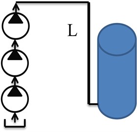
Next we represent the oil pumping system by a pipeline (Fig. 1) and its dynamic model (Fig. 2). The hydrodynamic system being analyzed consists of centrifugal pumps and a long pipeline (Fig. 2).

Fig. 1Altitude of oil transportation system

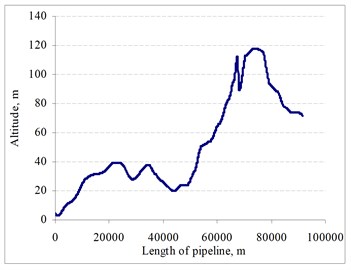
Fig. 2Hydrodynamics system

The equation of the fluid continuity can be written in a differential form as follows:

where $\rho$, $v$ are the density and velocity of the fluid, $S\left(x\right)$ is the cross section area of the pipeline, $F_1\left(x\right)$ is the discharge of the fluid mass to the unit of length in the pipeline. The equation of the fluid flow impulse (momentum):

where $p$ is the fluid pressure, $\mathrm{\Pi }\left(x\right)$ is the perimeter of the cross section of the pipeline, $\tau$ is the tangential fluid stress in the inner surface of the pipeline, $a_x$ is the acceleration along the $x$ axis, $F_2\left(x\right)$ is the kinetic energy of the fluid flow in the pipeline to the unit of area. The tangential fluid stress in the inner surface of the pipeline is determined:

Anti-turbulent fluid additives reduce the friction coefficient $\lambda$. This coefficient can be calculated from the equation [11]:

where $\theta$ is the concentration of the turbulent additives.

The friction coefficient $\lambda$ is determined by solving the nonlinear algebraic equation:

This equation is solved by the Newton-Raphson method:

The dependence of hydraulic resistance coefficient $\lambda$ on the Reynolds number and the FLO-XL additive concentration is presented in Fig. 3.

Fig. 3Dependence of hydraulic resistance coefficient λ on the Reynolds number and the FLO-XL additive concentration

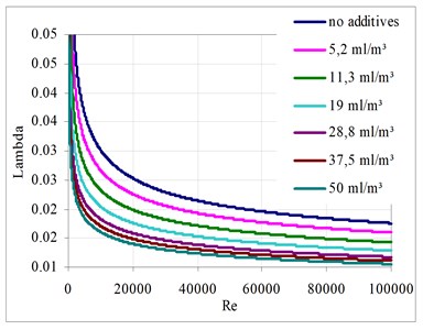
Fig. 4Dependence of coefficient k on the FLO-XL additive concentration

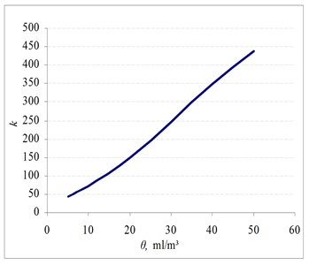
The results obtained from the calculation (Table 1) showed the dependence:

$k\left(\theta \right)=28.21+2.052\cdot \theta +0.246\cdot {\theta }^2-2.469\cdot {10}^{-3}\cdot {\theta }^3,$ which is given in Fig. 4.

The system of equations (1) and (2) can be written as a system of second-order quasi-linear differential equations:

where $\left[A\right]$, $\left[B\right]$ are matrices and $\left\{f\right\}$ is a vector which depends on $t$, $x$ and the elements $u_i$ of vector ${\left\{u\right\}}^{\mathrm{T}}=[p,v]$:

Equating the determinant of matrix $\left[B\right]-\left[A\right]\frac{dx}{dt}$ to zero, the equation which allows determination of the $\frac{dx}{dt}$ derivative and characteristic direction is obtained. This equation has two various real roots $dx/dt={\lambda }_i$, $(i=1,2):$

$a$ – the sound velocity in a liquid with a certain amount of gas, which is stored in an elastic pipeline, is equal to:

where: $K\left(p\right)$ – bulk modulus of the elasticity of the liquid, $\rho$ – density of the liquid, $E$ – modulus of elasticity of the pipeline,$\gamma$ – internal diameter of a pipeline, $e$ – thickness of the wall of a pipeline, $\gamma$ – index of adiabatic process, $\epsilon$ – ratio of the gas volume in the liquid and the total volume of the liquid (mixture).

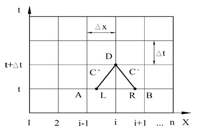
Differential equations of liquid movement in the pipeline are solved by the characteristics method [12]. The unknowns, variable velocity and pressure of the liquid at any specific moment in time $t+\Delta t$, are determined according to these parameters at the moment of time $t$ (Fig. 5). The length of the pipeline is divided into elements, the length of which is $\Delta x$. Pressure and velocity at a point $D$ at the moment of time $t$ are determined from the nonlinear algebraic equation system:

where: $f_1(v,p)=\frac{c_2}{S\left(x\right)}(F_1-\rho v\frac{\partial S}{\partial x})$; $f_2(v,p)=\frac{1}{\rho S\left(x\right)}(F_2-v{F}_1)-\frac{\tau \Pi \left(x\right)}{\rho S\left(x\right)}-a_x$; $\tau =\frac{\rho f\left(\mathrm{R}\mathrm{e}\right)v\left|v\right|}{8}$; $\lambda \left(\mathrm{R}\mathrm{e}\right)$ is the coefficient of pressure losses along the pipe; $\text{Re}$ is the Reynolds number.

The equation system was solved:

and the distributions of the initial pressure and velocity were determined.

This system of equations was solved by the finite element method and by using the Galerkin method.

Vector $\left\{u\right\}$ in the finite element is approximated by:

where: $\left[N\right(\xi \left)\right]=[1-\xi ,\xi ]$, $\xi =x/L_e$; $L_e$ – length of the finite element;

${\left\{q\right\}}_e^{\mathrm{T}}=\left[\begin{array}{cccc}{p}_{e1}& v_{e1}& p_{e1}& v_{e1}\end{array}\right].$

Fig. 5Scheme of determination of point parameters by characteristic method

The equation system for the finite element was determined by applying the Galerkin method:

or:

The general equation system of the oil pipeline was generated from the finite elements equation system (14):

The nonlinear equation system (16) was solved using the Newton-Raphson method:

The power of the friction force in the inner surface of the pipeline is equal:

The coefficient of efficiency of the pipeline is equal:

where $N_{input}$, $N_{output},$ are the power at the input and output of the pipeline, respectively.

3. Theoretical and numerical analysis

The main parameters of the investigated pipeline are the length of the pipeline $l=$ 91.6 km, outer diameter of the pipe $D=$ 0.559 m, wall thickness of the pipe $\delta =$ 0.0095 m and inner diameter of the pipe $d=$ 0.540 m. Temperature of the oil being pumped: highest during the summer, +25°C and lowest in the winter, –6°C. Efficiency of the system – 1400 m³/h, maximum admissible pressure in the pipeline – $P_{max}=$ 10.2 MPa. Density of the transported oil – 860 kg/m³ (at 20°C).

Oil pumping is done by six pumps with a nominal shaft rotation speed of 2980 rpm, powered by three-phase electric motors of 900 and 2000 kW with an efficiency of 0.96.

The general characteristic of the pumps and piping at the first pump intake pressure $H_p=$ 13.2 m are shown in Fig. 6. The horizontal line in Fig. 6 shows the pressure limit of the section of investigated pipeline. The intersection point of this line with the characteristic curve of the pump shows the lowest capacity at which the relevant number of pumps can operate.

The intersection points of the characteristic curves of the pumps and piping show the capacity of the hydraulic system and the pressure developed by the pumps. The pipeline capacity at any intersection point of the curves can be calculated by the formula:

where: $H_p$ – the inlet pressure of the first pump; $H_L$ – the pressure at a distance $L$ from the beginning of the pipeline; $z_L$ – position of geometric height; $a$ and $b$ – coefficients of characteristics; $\lambda$ – coefficient of resistance. The pipeline is divided into 18320 elements, the length of each pipeline element is $\Delta x$ = 5 m.

The selection of an appropriate integration time step $\Delta t$ is very important to the accuracy of the analysis. In this case, a time step of $\Delta t=$ 0.00025 s was selected for use in the integration process. The pressure and velocity at each pipeline point was obtained by solving a system of nonlinear algebraic equations. The system was solved by using the Newton-Raphson method. The duration of the hydrodynamic processes for this simulation was chosen to be 160 s. Initial pressure distribution along the pipeline is shown in Fig 7. Oil pressure and discharge at the corresponding pipeline points $x$ are shown in Fig. 8 to Fig 13.

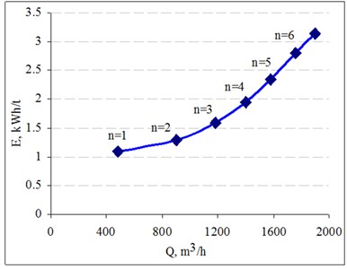
Oil pressure distributions after 160 s in the pipeline are shown in Fig. 14. The power of the friction forces in the inner surface of the pipeline with different concentrations of the additives are shown in Fig. 15. The efficiency coefficient of the pipeline is shown in Fig. 16 and the comparative energy dependency on oil pipeline productivity – in Fig. 17.

The relative energy costs of transporting one metric ton of oil decrease with increasing additive concentration.

Fig. 6General characteristic of the pumps and piping

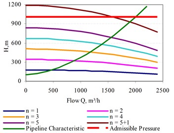
Fig. 7Initial pressure distribution in the pipeline

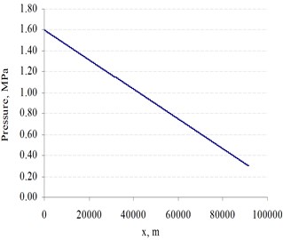
Fig. 8Dependencies of the pressure in the different pipeline points when concentration of additives in the oil is equal 0 ml/m3

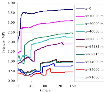
Fig. 9Dependencies of the discharge in the different pipeline points when concentration of the additives in oil is equal 0 ml/m3

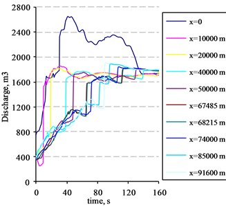
Fig. 10Dependencies of the pressure in the different pipeline points when the concentration of the additives in the oil is equal to 12 ml/m3

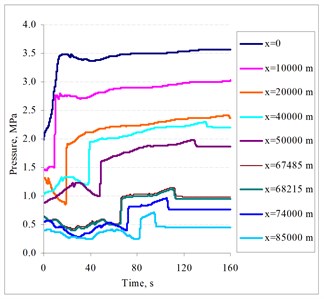
Fig. 11Dependencies of the discharge in the different pipeline points when the concentration of the additives in the oil is equal to 12 ml/m3

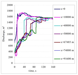
Fig. 12Dependencies of the pressure in the different pipeline points when the concentration of the additives in the oil is equal to 50 ml/m3

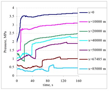
Fig. 13Dependencies of the discharge in the different pipeline points when the concentration of the additives in the oil is equal to 50 ml/m3

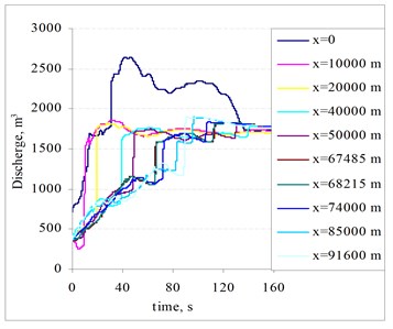
Fig. 14Distributions of pressure in the pipeline

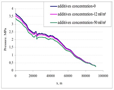
Fig. 15Dependencies of the power of friction forces in the inner surface of the pipeline

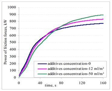
Fig. 16Dependencies of the pipeline efficiency coefficient

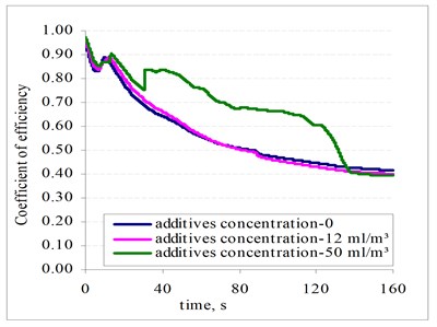
Fig. 17Comparative energy dependence on oil pipeline productivity

4. Conclusions

The methodology developed allows an assessment of the technological methods of oil transportation by pipelines in consideration of the usage of additives for the hydrodynamic processes.

A numerical simulation of the hydrodynamic system has shown that increasing the additive concentration in oil increases pipeline capacity and decreases the relative energy consumption. However, the cost for the oil additive amount in transporting one metric ton of oil increases.

The mathematical model and numerical analysis created enable the investigation of fluid transportation systems, the selection of optimal operation regimes, determination of the necessary number of pumps, and an evaluation of the anti-turbulent additives’ effects on optimal system performance.