Automatic artifacts removal from epileptic EEG using a hybrid algorithm

2.1. Data set

Scalp EEG recordings were collected from Zhejiang Provincial People's Hospital, China. The patients (12 females and 19 males, age: 32.8±7.7) acquired EEG inspection for diagnosis of epilepsy. Data acquisition system is Phoenix Unique Ambulatory EEG of EMS Handelsges.mbh Company, Austria. EEG signals are amplified with bandpass filter of 0.15–60 Hz and the sampling rate is set to 256 Hz. Exploring cup electrodes were fixed to the scalp at Fp1, Fp2, F3, F4, C3, C4, P3, P4, O1, O2, F7, F8, T3, T4, T5 and T6 according to the International 10–20 System, and the reference electrodes are located on the ipsilateral ear electrodes. Video recordings are acquired synchronously with EEG, by which artifacts such as EOG (e.g. eye blinks) and EMG (e.g. chewing) can be identified. All the subjects give informed consent.

2.2. Methods

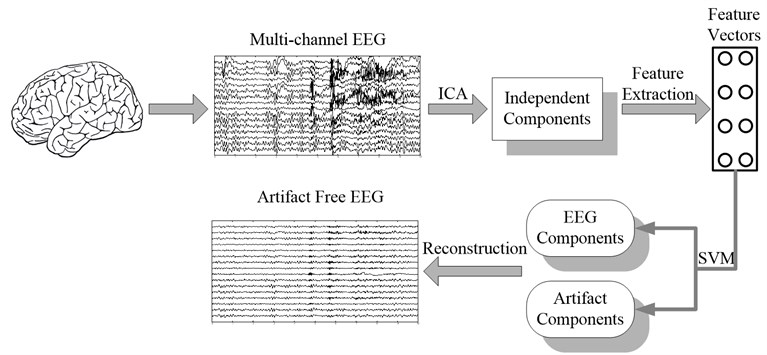
The fundamental procedure of artifact removal in EEG using ICA-based algorithm consists of three steps: (1) decompose the raw EEG into statistically independent components; (2) identify the artifact components; (3) eliminate the artifact components and reconstruct the signal with the remaining components. The key problem in automatic removal of artifacts is to identify the artifact components automatically. Here statistical features of the components in time and frequency domain are extracted and input into support vector machine to achieve the goal. The flow chart of automatic artifacts removal algorithm is shown in Fig. 1.

Fig. 1Block diagram of automatic artifacts removal with ICA and support vector machine

2.2.1. ICA

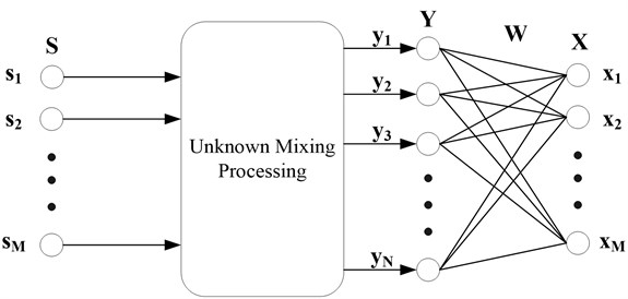
ICA [10] is a signal processing technique which aims at expressing a set of random variables as linear combinations of statistically component variables. It was originally proposed by Comon [11] to solve the BSS problem. The architecture of the problem is illustrated in Fig. 2, where $\mathbf{S}$ is the unknown source signal and $\mathbf{Y}$ is the observed signal collected with $N$ sensors. $\mathbf{X}$ is the approximation of the unknown sources acquired with the de-mixing matrix $\mathbf{W}$ and the observed signal $\mathbf{Y}$.

Fig. 2Architecture of BSS problem

In this paper we apply FastICA algorithm [12] to decompose the acquired EEG data into statistically independent components, using EEGLAB platform [13] running on MATLAB (The Mathworks, Natick, Massachusetts). It works on a non-overlapping window with length of 30 s, which contains sufficient samples to reliably separate the artifact from real EEG activities [8, 14]. The number of extracted independent components is equal to the number of recording electrodes [8]. Some independent components are probably a mixture of EEG and artifactual activities and extracting the features using the entire component may obscure the artifact segments. Thus we partition each 30 s component into six 5 s epochs.

2.2.2. Feature extraction

With ICA, artifacts and EEGs are separated into different independent components. Traditionally the identification of artifact components is achieved manually by observing the scalp maps and the fuzzy characteristics (in time and frequency domain) of the components. In order to identify the artifact segments automatically, we need to define quantitative features that can discriminate the artifact components from the EEG components. Here features in time and frequency domain, including Hurst exponent, skewness, Kurtosis, largest Lyapunov exponent and frequency-band energy, are selected.

Hurst exponent. Hurst exponent was first proposed by Hurst in 1965 [15]. It is used to evaluate the long-range dependence of a time series. Hurst exponent is usually calculated by the recurrent method [9] and ranges from 0 to 1. $\mathrm{H}=0.5$ corresponds to a standard Brownian movement, and $0<\mathrm{H}<0.5$ indicates the anti-persistent behavior, while $0.5<\mathrm{H}<1$ describes a temporally persistent or trend reinforcing time series. Obviously linear electrode artifact (e.g. baseline drift) has higher Hurst exponent than that of EEGs because of longer persistence. Furthermore extensive computer experiments show that artifacts such as eye blinking and heart beats have lower Hurst exponent than that of EEGs [9].

Skewness. Skewness corresponds to the third-order statistic of the data. An EEG recording that contains eye blink or baseline drift typically has a positive or negative skewness since the eye blinking artifact or the baseline drift artifact increases locally the asymmetry of the signal [16]. Here we take the absolute value of the skewness. As a result, the eye blink and baseline drift have larger skewness than that of normal EEGs, which are approximately symmetrically distributed.

Kurtosis. Kurtosis is the 4th cumulant of a time series, which quantifies how outlier-prone a distribution is [4]. Highly positive kurtosis indicates that the distribution of the signal is peak and sparse, and the identified activity is probably to be an artifact such as eye movements or ECG. The kurtosis of the normal distribution is 3, while the kurtosis of a periodical series is negative and the kurtosis of Gaussian noise is close to 0.

Largest Lyapunov exponent. Lyapunov exponent is a quantitative measure of the sensitive dependence on the initial conditions, which defines the average exponential rate of the divergence or convergence of the nearby orbits in the phase space. Specifically LLE is very useful in recognizing some basic rhythms that exist periodically in normal EEGs, as well as rhythmic seizure onsets in epileptic EEGs. When calculating LLE of EEG signals, an embedding dimension between 5 to 20 and a delay of 1 are proper [17]. In this paper we set the embedding dimension to 10 and delay to 1.

Frequency-band energy. Besides the above mentioned features in time domain, features in frequency domain are also useful, i.e. some of the artifacts have unique frequencies. Here we employ sub-band energy based on wavelet packet decomposition as features in frequency domain.

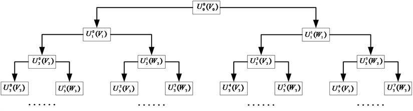
First each epoch is filtered between 0.3 and 60 Hz with a 10th order digital Butterworth. Then Wavelet Packet Decomposition (WPD) is applied to split the epoch into two orthonormal subspaces $V$ and $W$, where $V$ and $W$ include low and high frequency information of the original epoch, respectively. With multi-level decomposition, WPD leads to a complete wavelet packet tree, shown in Fig. 3. Thereinto, $U_{j,n}$ is the$n$th ($n$ is the frequency factor, $n=\mathrm{0,1},2,\cdots ,2j-1$) subspace of wavelet packet at $j$th scale, and $U_{j,k}^n\left(t\right)=2^{-j/2}{u}^n(2^{-j}t-k)$ indicates the corresponding orthonormal basis ($k$ is the shift factor), which satisfies with:

1

$u_{j,0}^n\left(t\right)=\left\{\begin{array}{c}\sum _k{h}_0\left(k\right)u_{j-1,k}^i\text{\hspace{0.05em}\hspace{0.05em}\hspace{0.05em}\hspace{0.05em}\hspace{0.05em}\hspace{0.05em}\hspace{0.05em}\hspace{0.05em}\hspace{0.05em}if\hspace{0.05em}\hspace{0.05em}\hspace{0.05em}}n\text{\hspace{0.05em}\hspace{0.05em}\hspace{0.05em}is\hspace{0.05em}\hspace{0.05em}\hspace{0.05em}even,}\\ \sum _k{h}_1\left(k\right)u_{j-1,k}^i\text{\hspace{0.05em}\hspace{0.05em}\hspace{0.05em}\hspace{0.05em}\hspace{0.05em}\hspace{0.05em}\hspace{0.05em}\hspace{0.05em}\hspace{0.05em}if\hspace{0.05em}\hspace{0.05em}\hspace{0.05em}}n\text{\hspace{0.05em}\hspace{0.05em}\hspace{0.05em}is\hspace{0.05em}\hspace{0.05em}\hspace{0.05em}odd,\hspace{0.05em}\hspace{0.05em}}\end{array}\right.$

where $j,k\in Z,n=\mathrm{0,1},2,\cdots ,2^j-1$, $h_0\left(k\right)$ and $h_1\left(k\right)$ are a couple of quadruple mirror filters (QMF) which are irrelevant to scales and satisfy with:

2

$h_1\left(k\right)={(-1)}_{1-k}{h}_0(1-k).$

The coefficient of WPD at $j$th level and $k$th sample can be calculated with:

3

$d_j^m\left(k\right)=\left\{\begin{array}{c}\sum _m{h}_0(m-2k)d_{j-1}^{n/2}\left(m\right)\text{\hspace{0.05em}\hspace{0.05em}\hspace{0.05em}\hspace{0.05em}\hspace{0.05em}\hspace{0.05em}\hspace{0.05em}\hspace{0.05em}\hspace{0.05em}\hspace{0.05em}\hspace{0.05em}\hspace{0.05em}\hspace{0.05em}\hspace{0.05em}\hspace{0.05em}\hspace{0.05em}\hspace{0.05em}if\hspace{0.05em}\hspace{0.05em}\hspace{0.05em}}n\text{\hspace{0.05em}\hspace{0.05em}\hspace{0.05em}is\hspace{0.05em}\hspace{0.05em}\hspace{0.05em}even,}\\ \sum _m{h}_1(m-2k)d_{j-1}^{(n-1)/2}\left(m\right)\text{\hspace{0.05em}\hspace{0.05em}\hspace{0.05em}\hspace{0.05em}\hspace{0.05em}\hspace{0.05em}\hspace{0.05em}\hspace{0.05em}\hspace{0.05em}if\hspace{0.05em}\hspace{0.05em}}n\text{\hspace{0.05em}\hspace{0.05em}\hspace{0.05em}is\hspace{0.05em}\hspace{0.05em}\hspace{0.05em}odd.\hspace{0.05em}\hspace{0.05em}}\end{array}\right.$

When we decompose the signal to $j$th level, the frequency ranges of all the subspaces are $\left\{\right[0,f_s/2^{j+1}],[f_s/2^{j+1},2f_s/2^{j+1}],[2f_s/2^{j+1},3f_s/2^{j+1}],\cdots ,[(2_j-1)f_s/2^{j+1},f_s/2\left]\right\},$ where $f_s$ is the sampling frequency. For a selected sub-band, its energy can be obtained by:

4

$E_{j,n}=\sum _k{\left(d_j^n\right(k\left)\right)}^2.$

Fig. 3Wavelet packet decomposition tree

Previous researchers show that significant power at low frequencies might suggest the presence of ocular or movement artifacts, while the power in the high-frequency band would indicate EMG contamination [8]. Furthermore some basic rhythms in EEG have specific frequency ranges and can be identified with frequency-band energy. In this paper we select Daubechies Wavelet (db4) [18-19] to decompose each 5 s epoch to 4-level wavelet packet and calculate the sub-band energy of 0~3.75 Hz, 3.75~15 Hz, 15~30 Hz, 30~60 Hz, namely, $\{E_{\mathrm{4,0}},E_{\mathrm{4,1}}+E_{\mathrm{3,1}},E_{\mathrm{2,1}},E_{\mathrm{1,1}}\}$ as the features in the frequency domain.

3.1. Training the algorithm

The acquired EEG signals are first decomposed into independent components using ICA. Each independent component is partitioned into six 5 s epochs. Features including Hurst exponent, skewness, kurtosis, largest Lyapunov exponent and frequency-band energy, are then calculated and input into support vector machine for classification. Altogether we have 16×16×10×2 = 5120 independent components (or 16×16×10×2×6 = 30720 5 s epochs) to train the support vector machine. 15360 epochs are selected as training set while others are test set. In the training set there are 6324 epochs containing different types of artifacts and 9036 free of artifact. The artifact epochs include 72 power frequency interference, 1266 EOG, 4481 EMG, 116 ECG and 389 baseline drift. In the test set 5100 epochs containing artifacts and 10260 free of artifacts are involved. The artifact epochs contain 31 power frequency interference, 932 EOG, 3938 EMG, 60 ECG and 139 baseline drift.

The average error of the support vector machine is estimated as follows. Firstly 1280 independent components (7680 epochs) of the training set are randomly selected as training samples and 1280 independent components (7680 epochs) of the test set are randomly decided as test samples. Two experienced clinicians are asked to review all the independent components to decide whether it is artifact or not. Feature vectors of the training samples are then calculated to train the support vector machine and the support vectors of the support vector machine are obtained. After that feature vectors of the test samples are calculated and input into the trained support vector machine for classification. The sum of epochs representing artifacts is then used to determine whether to reject or preserve each independent component. A threshold $T_h$ is chosen to get minimum classification error. If the threshold is too high, some artifacts are probably preserved. If the threshold goes too low, lots of normal EEGs will be lost [8]. Besides the threshold, two important parameters in support vector machine, $C$ and $\sigma$, have a decisive effect on the classification accuracy [16]. In order to find the optimal $T_h$, $C$ and $\sigma$, we calculate the average of classification error with a predefined range of these parameters. The above process is performed ten times to yield average of the classification error. The optimal $T_h$, $C$ and $\sigma$, which correspond to the lowest classification error, are found to be 4, 500 and 7, respectively. With the optimized parameters we obtain an average training error of 4.91 % and the average number of support vectors is 13.2 % of the training data set size.

3.2. Testing the algorithm

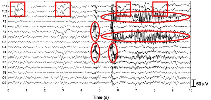
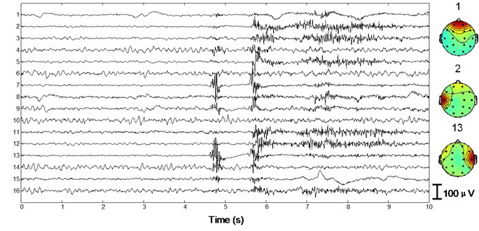
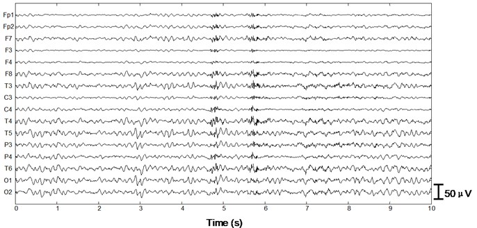
We apply the algorithm with optimal parameters to the validation set (15 patients). After ICA we obtain 15×16×10×2 = 4800 independent components with duration of 30 s. First a typical performance of the proposed method on normal EEG is shown in Figure 4. Since 30 s window is too compressed to depict low-frequency information of the EEG data as well as the independent components, we only draw 1/3 in length, i.e. 10 s. In Fig. 4(a) 10 s EEG is contaminated by artifacts in numerous channels. Four eye blinks occur at 0.5 s, 2.8 s, 6.2 s and 8 s on Fp1 and Fp2, respectively (see the square boxes). Besides obvious EMG artifacts can be found at 4.8 s on F8, 5.6 s on F7 and T3, 4.8 s and 5.6 s on T4, respectively (see the ellipses). P3, P4, O1 and O2 are also slightly contaminated by EMG artifacts. Fig. 4(b) shows the decomposed independent components. We can find eye blink features on IC1, which is also demonstrated in the scalp map. Obvious EMG artifacts exist on IC2, IC3, IC5, IC7, IC11, IC12 and IC13. For example, scalp maps show that IC2 includes movement artifact on the left hemisphere, while IC13 indicates chewing artifact on the right. Besides IC8, IC15 and IC16 are also identified as artifact components by our algorithm. The signals are reconstructed with the remaining independent components, i.e. IC4, IC6, IC9, IC10 and IC14, shown in Fig. 4(c). We can still find very few chewing artifacts at 4.8 s and 5.6 s on F8, T3, T4 and T6. Previous studies also show that it is rather difficult to remove chewing artifacts completely since they spread in numerous channels with large amplitude. Note the scale difference between Fig. 4(a), (b) and (c).

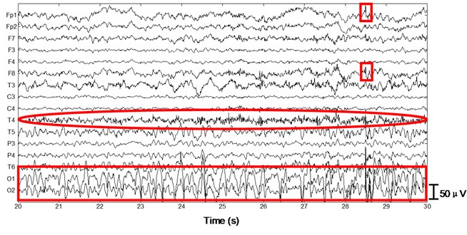
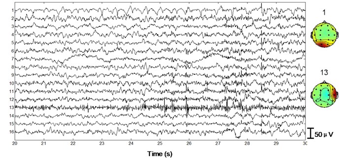
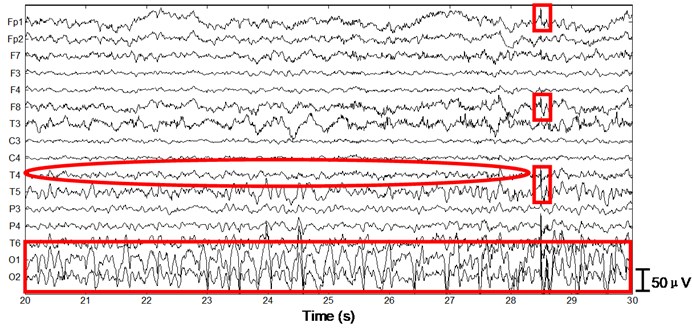
Next we apply the proposed method to ictal EEG, shown in Fig. 5. Ictal events on O1 and O2 (see the big square box) shown in Fig. 5(a) and simultaneous video recordings confirm an occipital seizure. Epileptic spike waves are also presented at 28.5 s on Fp1 and F8 (see the small square boxes). EMG artifacts exist on T4 throughout the 10 s window (see the ellipse). The decomposed independent components are shown in Fig. 5(b). IC13 is composed of muscle artifacts. With the scalp map it can be concluded as movement artifacts on the right hemisphere. In addition, with the scalp map as well as the waveform of IC1, we believe IC1 is a rhythmic activity on occipital area, which is also to be confirmed by calculating the LLE of IC1 (–0.2235). Reconstructed EEGs are shown in Fig. 5(c). EMG artifacts on T4 are removed completely, while ictal events on O1 and O2 are fully retained. Meanwhile epileptic spike waves on Fp1 and F8 are preserved and a spike wave on T5 which is not marked in Fig. 5(a) is also detected.

The performance of the algorithm on the validation set is shown in Table 1 and the results are justified by two clinicians at Zhejiang Provincial People's Hospital. The global average classification error is 10.54 %. As stated before, in the training process, the training and testing samples are randomly selected from 16 patients. Though the two samples are non-overlapping, part of them are probably from the same patients, which indicates that they have similar characteristics. However, in the validation process, the validation set is from other 15 patients and independent from the training and testing samples. This is why the average testing error (10.54 %) is much higher than the average training error (4.91 %). Even so, it shows that the proposed method has promising generalization ability.

Besides the global classification error, we also measure the classification error of epileptic EEG components, which indicates the number of epileptic components that are removed. Thereinto, no epileptic components are removed in 3 out of 15 patients (patient #1, #9, #10). In patient #3, 10 out of 87 epileptic components are classified as artifacts. We explored the EEG recordings and found that these epileptic components are severely contaminated by heavy muscle artifacts during epileptic seizures. Further we scanned all the misclassified epileptic components for the remaining 11 patients and obtained similar results. Relatively, nearly all the epileptic components during interictal period are correctly classified. In general over 95 % epileptic components are retained, which demonstrates that the proposed method is an efficient tool in removing artifacts from epileptic EEGs.

Fig. 4Performance of the algorithm on interictal EEG

a)

b)

c)

Fig. 5Performance of the algorithm on ictal EEG

a)

b)

c)

4.1. Discussion

A very important issue is the partition of independent components. In the proposed method feature vectors are calculated based on the partitioned epochs of independent components (30 s). This is very important because some independent components are a mixture of EEG and artifacts. Extracting the features using the entire independent component may obscure the artifact segments. On the other hand, the length of partitioned epoch is a key issue. If the partitioned epoch is too short, the computational load will increase substantially. Meanwhile this will also lead to the high probability of partitioning low-frequency artifacts into different epochs, which obscures the artifact features and eventually affects the classification accuracy [8]. After exploring the common artifacts in EEG, we decide that 5 s epoch is enough to describe the characteristics of the artifacts.

4.2. Conclusion

In this paper we have presented a robust method for removing artifacts from epileptic EEG based on ICA and SVM. ICA is used to decompose the acquired EEG data into independent components. Each independent component is then partitioned into 5 s epochs. With the predefined eight features in time and frequency domain, including Hurst exponent, skewness, kurtosis, largest Lyapunov exponent and frequency-band energy, the artifact epochs can be automatically identified with the trained support vector machine. The sum of epochs representing artifacts is then used to determine whether to reject or preserve each independent component. Artifact-free EEGs are reconstructed with the remaining independent components. Results show that the proposed algorithm can identify and remove a variety of artifacts in interictal and ictal EEGs, such as baseline drift, ECG, EMG, EOG and power frequency interference. Compared with traditional automatic artifact removal methods [7, 20], the proposed algorithm in this paper does not require reference channels (e.g. ECG, EOG), which would be more appropriate for clinical EEG data.