Time-frequency feature extraction from multiple impulse source signal of reciprocating compressor based on local frequency

1. Introduction

Reciprocating compressor plays an important role in petrochemical industry. Once the key parts of reciprocating compressor fail, considerable economy losses and serious safety problems will arise. So it is of great significance to monitor and diagnose the faults of reciprocating compressor. Feature extraction of signal is the priority process of machinery fault diagnosis. Vibration signals generated by reciprocating compressor present a multiple impulse source property, which is typical non-stationary [1]. Conventional signal processing techniques include time-domain statistical analysis and Fourier transform, which have proved to be effective in fault diagnosis of rotating machinery. However, these techniques are based on the assumption that the process of signals is stationary and linear, and they usually result in false information when applied to the non-stationary signal [2-3].

To process the non-stationary signal, time-frequency analysis techniques, such as short time Fourier transform (SFTF) [4], Wigner-Ville transform (WVT) [5-6], wavelet transform (WT) [7-8] and Hilbert-Huang transform (HHT) [9-11], have been widely applied to fault diagnosis of rotating machinery, which attracted more and more attention during the past few decades. However, all of them also present some limitations. In the case of the STFT, a good frequency resolution needs a long sliding window and therefore leads to a bad localization in time and vice versa, so the window length has to be chosen based on a prior knowledge of the signal [12]. Although WVT has good resolution in both time and frequency, its cross-terms cause some false information for multi-component signal [13]. Compared with STFT and WVT, WT is much better and widely used in time-frequency analysis. However, WT still has some inevitable deficiencies. Firstly, energy leakage will occur when using wavelet transform to process signals due to the fact that wavelet transform is essentially an adjustable windowed Fourier transform. Secondly, the appropriate base function needs to be selected in advance. Moreover, once the decomposition scales are determined, the result of wavelet transform would be the signal under a certain frequency band. Therefore, wavelet transform is not a self-adaptive signal processing approach in nature [14]. Hilbert-Huang Transform (HHT) as an adaptive time-frequency analysis technique has been developed and widely applied in many fields [15], which is demonstrated to be superior to WT analysis in many applications [16]. By HHT, the frequency and energy distribution of signals can be obtained from the instrinic mode functions (IMFs). Because the decompostion level of IMF is uncertain and uncontrollable, HHT often produces some unknown or even false frequency components of investigated signals.

At present, the work on frequency is focused on two concepts: traditional frequency (TF) and instantaneous frequency (IF). Thereinto, TF has been well known for the Fourier spectral analysis, which is defined for the period function spanning the whole data length of signal with constant amplitude [17]. Time-frequency analysis techniques, including the SFTF, WVT and WT, are all based on the concept of TF, and it can only show some meaningful explanations for periodic signal [18]. To analyze the non-periodic signal, IF is better than TF, and it is defined as the derivative of phase for arbitrary signal, which gives one frequency value corresponding to any instantaneous time [19]. Although IF obtained by HHT has been widely used in many fields for recent years, the existence of a meaningful IF is still highly controversial [20]. It seems that IF only represents the existence of frequency at one instantaneous time, which has no correlation with data information in the past or future. In practice IF needs the whole length of data.

To overcome the issue above, a novel concept of local frequency (LF) is proposed in the paper, which is an extention of TF and IF. Based on the concept, a time-frequency distribution approach and its algorithm are established. To identify the feasibility and effectiveness of the proposed approach, some non-stationary simulation signals, such as multi-harmonic signal, FM signal and multiple impulse source signal are analyzed. Compared with WVT, WT and HHT, time-frequency analysis based on LF can extract features of non-stationary signal more clearly and accurately. Moreover, the proposed approach is applied to the fault feature extraction of reciprocating compressor gas valve vibration signal in normal valve state and gap valve state. The results indicate the superiority of proposed approach in extracting time-frequency features from multiple impulse source signal of reciprocating compressor, which obtains a more precise result than WVT, WT and HHT. So it can provide an effective basis to fault diagnosis of reciprocating compressor.

2. Definition of LF

The definitions of TF and IF have been well known at present. TF for an arbitrary signal $x\left(t\right)$ can be obtained by Fourier transform, which is [21]:

where $f$ is TF, and the unit is denoted by Hz.

Moreover, IF for an arbitrary signal $x\left(t\right)$ can be expressed by Hilbert transform as [22]:

where $\omega$ is IF, and the unit is denoted by rad/s.

According to the definition of TF and IF, a novel concept of LF is proposed, which is defined based on the principle of three scales as follows.

1) Time scale: define the beginning and end time of period of time, denoted by $T_s$.

2) Peak scale: define the minimum and maximum of peak, denoted by $P_s$.

3) Time interval scale: define the minimum and maximum of adjacent peak interval, denoted by ${\Delta }_s$.

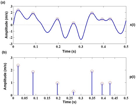
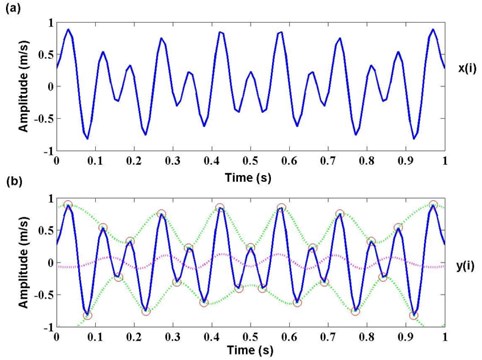
As is known to all, peak can represent the ultimate state of vibration signal in a period. Thus, it also can be used as the beginning or the end flag of each period. For an arbitrary time series of zero mean normalization $x\left(i\right)$, $(i=1,2,\dots ,n)$, its peak series $p\left(i\right)$, $(i=1,2,\dots ,n)$ can be obtained by equation (3). Fig. 1 shows the generation process of peak series $p\left(i\right)$ from $x\left(i\right)$:

Fig. 1Generation process of peak series p(i) from time series x(i)

Then, the time scale $T_s$ and peak scale $P_s$ of time series $x\left(i\right)$ can be given by:

where $a$ is time scale factor, representing the different time range of $x\left(i\right)$ and $b$ is peak scale factor, indicating the different peak range of $x\left(i\right)$. $F_s$ is sample frequency.

Generally, the selection of parameters $a$ and $b$ are arbitrary, which mainly depend on the characteristic of time series $x\left(i\right)$. Fig. 2 shows the definition process with different time scale and peak scale of $x\left(i\right)$.

In equation (3), the non-zero points of $p\left(i\right)$ indicates the peak variety of $x\left(i\right)$. Its subscript can be defined as flag series $f\left(j\right)$, $(j=1,2,\dots ,m)$, and each interval of two adjacent non-zero points of $p\left(i\right)$ can form into a series $\Delta \left(k\right)$, $(k=1,2,\dots ,l)$, that is:

Then, time interval scale ${\Delta }_s$ can be given by:

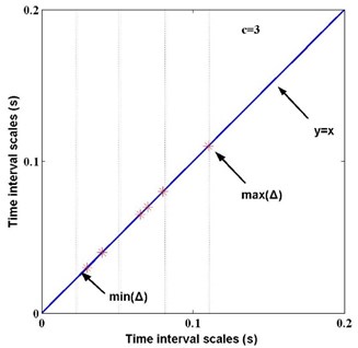
where $c$ is interval scale factor, representing the different time interval range of adjacent peak. As an example, Fig. 3 shows the calculation process of interval series $\Delta \left(k\right)$ when time scale $a=$ 1 and peak scale $b=$ 1. Assuming that $c=$ 3, it means that time interval is divided into three sections, which indicates the different scale levels. Each time interval belongs to corresponding section, and the principle is shown in Fig. 4.

Fig. 2Definition process with different time scale and peak scale of time series x(i)

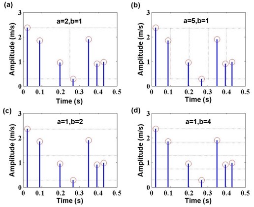
Fig. 3Calculation process of interval series Δ(k) when a= 1 and b= 1

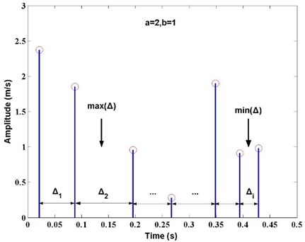
Fig. 4 illustrates the number of time interval in different sections can be counted, and then the repeating time interval is chosen for calculating LF. If there is no repeating time interval each other in a district, all of the time interval will be considered as almost-repeating time interval LF. Assuming that the statistic number of repeating or almost-repeating time intervals in each corresponding section is $N_s$, LF can be obtained as follows:

where $\upsilon$ represents LF, which measures the number of periods per unit time. And $t^{*}$ is the local time of investigated time intervals.

Fig. 4Principle of time intervals belonging to different sections when c= 3

3. Establishment of time-frequency distribution based on LF

A time–frequency distribution is a signal representation in which time, frequency and energy (or amplitude) are displayed jointly on a 2-D plane. According to the definition of LF above, the local time and LF information can be obtained in equation (9). Moreover, the local energy can be calculated as follows:

where $T$ is local period; the local energy $a$ reflects the scale of fluctuation with LF $\upsilon$.

Then, for an arbitrary time series of $x\left(i\right)$, $(i=1,2,\dots ,n)$, the algorithm of time-frequency distribution based on LF can be established as the following steps.

1) Initialize: let $r\left(i\right)=x\left(i\right)$, $k=$ 1.

2) Identify time points corresponding to all local maxima and local minima of $r\left(i\right)$, designated as $t_{\mathrm{m}\mathrm{a}\mathrm{x}}\left(i\right)$, $(i=1,2,\dots ,n)$ and $t_{\mathrm{m}\mathrm{i}\mathrm{n}}\left(i\right)$, $(i=1,2,\dots ,m)$ respectively. $n$ is the number of local maxima and $m$ is the number of local minima. According to equation (9), computing the LF ${\upsilon }_{\mathrm{m}\mathrm{a}\mathrm{x}}\left(i\right)$ and ${\upsilon }_{\mathrm{m}\mathrm{i}\mathrm{n}}\left(i\right)$, i.e.:

Therefore, all the LF for local maxima and local minima of $r\left(i\right)$ can form two LF vector $V\left(k\right)$ and $V(k+1)$:

Similarly, according to equation (10), two local energy vetrors $A\left(k\right)$ and $A(k+1)$ can also be obtained:

3) Connect all the local maxima by a cubic spline interpolation to form upper envelope and all the local minima to form lower envelope, and obtain a new time series $y\left(i\right)$ by the envelope mean; the envelop process of time series $y\left(i\right)$ from $x\left(i\right)$ is shown in Fig. 5.

Fig. 5Envelope process of time series y(i) from x(i)

4) Compute standard derivation and the number of extremum for time series $y\left(i\right)$, and then the calculation will be stopped when $y\left(i\right)$ meets one of the following conditions. Otherwise, let $r\left(i\right)=y\left(i\right)$, $k=k+2$ and return to the step 2).

i) The standard deviation of $y\left(i\right)$ is smaller than given threshold value which is about 0.001.

ii) The number of local maxima and local minima of $y\left(i\right)$ are both less than 2.

5) Finally, LF matrix $M_V$ and local energy matrix $M_A$ can be expressed respectively as follows:

Both LF matrix $M_V$ and local energy matrix $M_A$ are functions of local time, therefore the time-frequency distribution based on LF can be obtained by plotting the energy matrix in the time-frequency plane.

4. Evaluation of performance

Before applying the proposed time-frequency technique based on LF to multiple impulse source signals of reciprocating compressor, we need test its feasibility and accuracy on some non-stationary simulation signals, for which the ground truth is fully known. The simulated signal is selected as multi-harmonic signal, FM signal and multiple impulse source signal, whose characteristics are much closer with those of reciprocating compressor signals. Moreover, the time-frequency techniques, such as WVT, WT and HHT, are applied to compare the performance of proposed time-frequency technique.

1) Simulation with multi-harmonic signal:

where time $t=$ 0~1 s, sample frequency is 1000 Hz, and amplitude unit is m/s.

It is obvious that the original frequency components include 40 Hz and 10 Hz. In addition, the former energy is higher than the latter. The waveform of multi-harmonic signal is shown in Fig. 6. According to the algorithm of novel time-frequency distribution based on LF above, with the application of WVT, WT and HHT to the feature extraction of multi-harmonic signal, the result is shown in Fig. 7.

Fig. 6Waveform of multi-harmonic signal

In Fig. 7, although all the time-frequency features of multi-harmonic signal based on WVT, WT, HHT and LF can reflect the original frequency components 40 Hz and 10 Hz, the analysis result of each time-frequency technique also present some differences together. The feature with WVT contains a cross-frequency component 25 Hz, which is the mean of 40 Hz and 10 Hz. The feature with WT has no cross-frequency, but the frequency resolution is worse than WVT. The feature with HHT is superior to WT, but it also produces some unknown frequency informations near 10 Hz. Compared with WVT, WT and HHT, the proposed time-frequency distribution based on LF suggests the best performance in both frequency representation and frquency resolution.

2) Simulation with FM signal:

where time $t=$ 0~1 s, sample frequency is 1000 Hz, and amplitude unit is m/s.

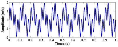
From equation (20), we can determine that the original feature frequency mainly contains two aspects: one is carrier frequency 50 Hz and the other is modulation frequency 10 Hz. Therefore the frequency range of FM signal is 40~60 Hz. Fig. 8 shows the waveform of FM signal. Apply the time-frequency analysis technique of WVT, WT, HHT and LF to the feature extraction of FM signal, and the result is shown in Fig. 9.

Fig. 7Time-frequency features of multi-harmonic signal with different techniques

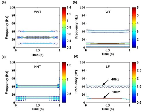
Fig. 8Waveform of FM signal

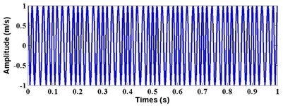
Fig. 9 represents a great difference in time-frequency features of FM signal with WVT, WT, HHT and LF. In the case of WVT, due to there existing many cross-frequency components, the original frequency feature of FM signal can not be recognized easily. The feature of WT indicates that there are three constant frequencies 40 Hz, 50 Hz and 60 Hz, which are original frequency components. Moreover, the frequency bands are much wider, so the resolution of WT is too bad. The feature with HHT is better than WVT and WT. It can clearly show the fluctuation of modulated frequency around carrier frequency. However, it also produces some unknown frequency information near 40 Hz and 60 Hz. The feature of proposed time-frequency distribution based on LF represents a quite consistent result and precise presolution of FM signal, which performs best in both frequency representation and frequency resolution.

3) Simulation with multiple impulse source signal:

where sample frequency is 1000 Hz, and amplitude unit is m/s.

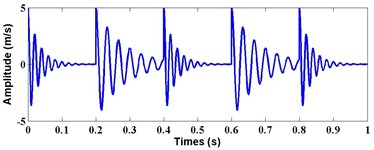
The simulated multiple impulse source signal is much similar as vibration signals of reciprocating compressor. It contains two kinds of impluse signals: one feature frequency is 50 Hz and corresponding attenuation frequency is 5 Hz. The other feature frequency is 30 Hz and corresponding attenuation frequency is 2 Hz. In addtion, the form respectively appears in the time of [0, 0.2] s, [0.4, 0.6] s and [0.8, 1] s. The latter respectively appears in the time of [0.2, 0.4] and [0.6, 0.8]. Fig. 10 shows the waveform of multiple impulse source signal. Moreover, Fig. 11 presents the time-frequency analysis technique of WVT, WT, HHT and LF to the feature extraction of multiple impulse source signal.

Fig. 9Time-frequency features of FM signal with different techniques

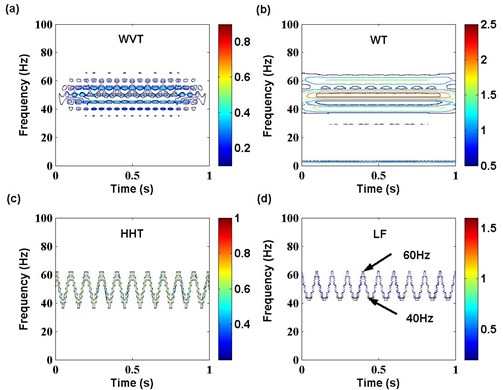
Fig. 10Waveform of multiple impulse source signal

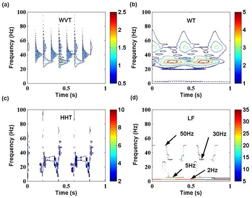
From Fig. 11, only WT and LF can effectively extract the frequency feature of multiple impulse source signal. In the case of WT, it can detect the frequency components around 30 Hz and 50 Hz, which are the original frequency feature of signal. However the attenuation frequency components can not be reflected, and the resolution of WT is much worse. The feature of LF presents the best characteristics among the four time-frequency analysis techniques. Not only can it extract the original frequency components 30 Hz and 50 Hz, but also detect the attenuation frequency components 2 Hz and 5 Hz. For the feature of WVT and HHT, there exist many cross-frequency or false frequency components, so they are not suitable to be used to analyze this kind of signal, which is much similar as multiple impulse source signal of reciprocating compressor.

4) Discussion.

In summary, the proposed time-frequency analysis technique based on LF is feasible and effetive in feature extration of non-stationary signals. It shows more meaningful frequency components of signals. Compared with WVT, WT and HHT, LF can obtain higer resolution and more accurate feature from the investiged signals, especially for the time-frequency analysis of mutiple impulse source signal. In addition, the simulation results indicate that each time-frequency technique has their own advantages, which is more suitable for analyzing some certain signals. Of course, so far there has been not any time-frequency technique which can process all kinds of signals. LF also has some limitations, such as the anti-noise performance and end effect, so it needs to be improved in the next work.

Fig. 11Time-frequency features of multiple impulse source signal with different techniques

5. Feature extraction from multiple impulse source signals of reciprocating compressor

In order to extract fault features of multiple impulse signals of reciprocating compressor, the reciprocating compressor gas valve is taken as the research object, and the vibtation data in two states including normal vale state and gap valve state are investigated by proposed time-frequency analysis technique based on LF [23]. Fig. 12 displays the experimental equipment installation for reciprocating compressor, and Fig. 13 shows the structure sketch of reciprocating compressor test-bed. Vibration signals were collected by vibration acceleration transducers fixed on gas valve cover. Sample frequency is 20000 Hz, and sample time is 0.1 s. Time waveform of gas valve vibration signal in four states is shown in Fig. 14.

The waveform of gas valve signals can only represent time information and amplitude information of some main impulsions. In normal valve state, the gas valve signal is detected in three main impulsions, which are respectively in 0.032 s, 0.05 s and 0.077 s. Among these impulsions, the highest amplitude appears in 0.05 s. In gap valve state, there are also three main impulsions, and they appear in 0.01 s, 0.03 s and 0.094 s respectively. Among these impulsions, the highest amplitude appears in 0.01 s. These features extracted from waveform of gas valve signal in two states are not enough to diagnose the faults of reciprocating compressor. To solve this problem, apply proposed time-frequency analysis technique based on LF to extract the feature of multiple impulse signals of reciprocating compressor. To indicate the superiority of proposed approach, time-frequency analysis techniques of WVT, WT and HHT are also applied to the investigation. The time-frequency features of gas valve signal in normal valve state and gap valve state with different techniques are respectively shown in Fig. 15 and Fig. 16.

Fig. 12Experimental equipment of reciprocating compressor gas valve

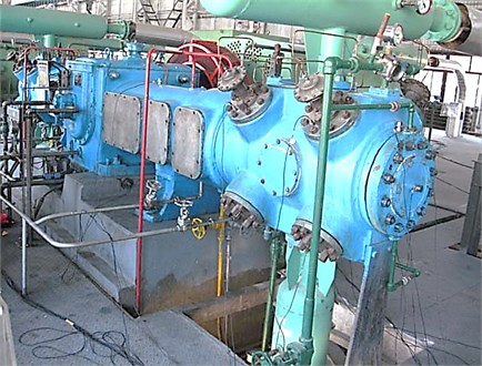
Fig. 13Structure sketch of reciprocating compressor test-bed

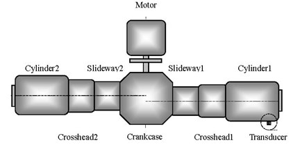
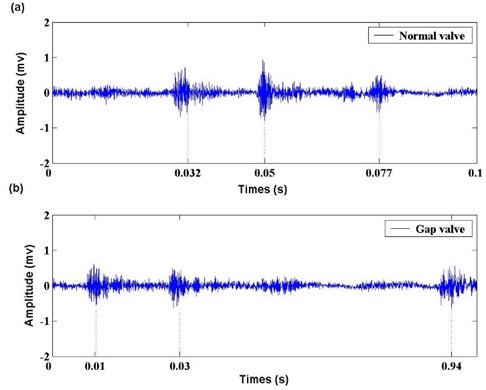
Fig. 14. Waveform of gas valve signals in two states

Fig. 15Time-frequency features of gas valve signal in normal valve state with different techniques

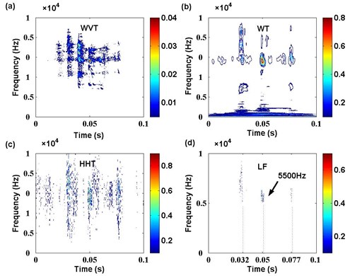
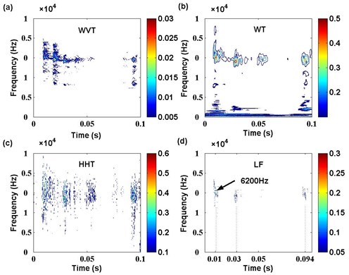
Fig. 16Time-frequency features of gas valve signal in gap valve state with different techniques

In the case of normal valve state shown in Fig. 15, although we can obtain that the highest energy component corresponding to 5500 Hz appearing in 0.05 s in each time-frequency feature of WVT, WT, HHT and LF, there also exist much difference in each result. As for the interference of cross-frequency, the feature of WVT can not easily detect the other two main frequency bands which should respectively appear around 0.032 s and 0.077 s. Compared with WVT, WT can reflect all main features mentioned above, but it can not obtain better resolution in both time scale and frequency scale. The performance of HHT is just as our previous analysis, which produces a lot of unknown frequency bands when impulse component appears. Therefore it is not suitable for feature extraction from multiple impulse signals of reciprocating compressor. The feature of LF represents the best characteristics than other time-frequency analysis techniques. It clearly shows that the three main frequency components respectively appear in 0.032 s, 0.05 s and 0.077 s, which matches the waveform analysis result above. Moreover, the three frequency bands are much narrower, so the time-frequency distribution based on LF propose a high resolution for the feature extraction from multiple impulse signals of reciprocating compressor.

In Fig. 16, the results further identify the similar performance of WVT, WT, HHT and LF for the feature extraction from multiple impulse signals of reciprocating compressor. The features of LF indicate the three main frequency band components respectively appearing in 0.01 s, 0.03 s and 0.094 s, which also matches the waveform analysis result above. Among these components, the highest frequency corresponding to 6200 Hz appears in 0.01 s. In addition, LF also proposes a high resolution, by which the different gas valve state can be well distinguished. So the analysis result can be effectively used in fault diagnosis of reciprocating compressor.

6. Conclusions

As for the limitation of current time-frequency analysis techniques based on TF or IF, the novel time-frequency distribution based on LF is proposed. Compared with the performance of WVT, WT and HHT on feature extraction of simulation signals, the feasibility and effectiveness of proposed approach are well identified. The investigation suggests that LF is more suitable for analyzing the multiple impulse source signals. With this method, the high resolution and accurate feature can be obtained. By applying the LF to fault feature extraction from multiple impulse source signals of reciprocating compressor in normal valve state and gap valve state, the results show the superiority of proposed approach in extracting time-frequency features from multiple impulse source signal of reciprocating compressor, which obtains a more precise result than WVT, WT and HHT. So it can provide an effective basis to fault diagnosis of reciprocating compressor.