Abstract
The short thin cylindrical shells are important component used in rotating machinery and its function is to connect shafts and transmitted torque. The kind of components is always destroyed due to vibrational state, so it is necessary to further research on the vibration characteristics. In this paper, the vibration characteristics of short thin cylindrical shells are solved using the beam function method, the transfer matrix method and the finite element method respectively. The solving results of three calculating methods are compared by simulation in the clamped-free and clamped-clamped boundary conditions. The simulation results show that the solving results of the transfer matrix method are close to the results of finite element method, but the deviation of the results of the beam functions method is larger than the other two methods. Furthermore, the experiments of the short thin cylindrical shell in the clamped-free boundary conditions are studied. The experimental results verify that the transfer matrix method and the finite element method are applicability to solve the vibration characteristics of the short thin cylindrical shells.
1. Introduction
Short thin cylindrical shell usually means that the axial half-wave number is 1, and the ratios of thickness and other minimum parameter (i.e. diameter and length) is between 1/80 and 1/5 [1]. The short thin cylindrical shell has grown in importance with the increasing use of shell structures for a wide variety of applications in aerospace, shipbuilding, chemical machinery and other branches of engineering. It is important component used in rotating machinery and its function is to connect shafts and transmitted torque. It is subjected to centrifugal force, aerodynamic force, and vibration alternating force and other load during its working. The kind of components is always destroyed due to vibrational state. So it is necessary to further research on the vibration characteristics.
Currently numerous studies have been made to understand the vibration characteristic of the short thin cylindrical shell. In order to calculate the inherent characteristic of cantilever cylindrical shell, the Rayleigh-Ritz method, the axis-symmetry finite element method and the exact analytic method are employed by C. B. Sharma and D. J. Johns [2-3]. By using of the Love’s shell equations, the influence of boundary conditions for a thin rotating stiffened cylindrical shell is researched by Lee [4]. Vibration characteristics of the laminated cylindrical shell are studied, then influence of boundary conditions and geometric parameters for system dynamics characteristics is analyzed by Zhang [5]. Studies for dynamic characteristic of boundary conditions for thin cylindrical shells have also been carried out by Lam and Loy [6]. Li Xuebin presents a new approach of separation of variables in circular cylindrical shell analysis for arbitrary boundary conditions [7]. The instant response of the laminated shell is subject to radial impacting loads and axial pressure load, and the boundary condition investigated in the study is clamped-simply. The analysis is carried out using Love-type shell theory and the first order shear deformation theory by Jafari and Hamid [8, 9]. However, many of these studies are restricted to theory analyses. Studies for the contrast test of different analyze methods are seldom attempted, especially the experimental tests.
In this paper, the vibration characteristics of short thin cylindrical shells are solved using three analytical methods which is the beam function method, the transfer matrix method and the finite element method respectively, and then using the results of experiment confirmed the correctness and validity of analysis methods.
2. Analysis based on the beam function method
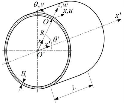
Figure 1 shows the nomenclature of a short thin cylindrical shell. The reference surface of the cylinder is taken at the middle surface where an orthogonal coordinate system () is fixed. The coordinates system () is the coordinates system () translate from origin along direction to one point of the middle surface. -axis and -axis are parallel and in the same direction. -axis and -axis are overlapping and in the same direction. -axis and -axis are overlapping. In the Figure 1, is the radius, is the length, is the thickness, is the material density, is the Young's modulus and is the Poisson's ratio. The deformations of the cylindrical shell in the , and directions are denoted by , and , respectively.
Fig. 1The structures of the thin-walled cylindrical shells
2.1. Dynamic functions
The dynamic functions for a short thin cylindrical shell which describe the vibration characteristics of the vertical, tangential and radial vibrate can be written as [10]:
where is the different membrane stiffness, is the flexural rigidity; , and are inertia item.
In terms of the displacements , and is derived for the free vibration of a rotating cylindrical shell and be written in the following form:
where are differential operators and can be written as follows:
2.2. Analytical method
The vibration mode functions of short thin cylindrical shell are derived for the axial beam function and the circumferential triangle function and can be written in the following form [10]:
where , and are the displacement amplitudes, and and are the axial and circumferential wave numbers, respectively. , , , , and are written as and .
The functions are circumferential modal functions, where are the natural frequencies. The functions are the axial modal functions. The functions are written as the beam functions which can be expressed in a general form as Eq. (6):
where , and are some constants with value depending on the boundary condition [11]. The parameters are given as follow for the following boundary conditions.
Table 1The parameters corresponding to boundary conditions
Boundary conditions | The parameters |
S-S | |
C-C | |
C-F | |
S-C |
The Eq. (5) is substituted into Eq. (4) and Galerkin’s method is applied. The Eq. (4) can be written as:
After performing the integration, Eq. (7) can be written in a matrix form as:
where are equation coefficients and can be written as:
where , and are defined as:
The Eq. (8) is solved by imposing non-trivial solutions condition and equating the determinant of the characteristic matrix to zero. A polynomial of the form can be obtained:
where are equation coefficients and can be written as:
Six are obtained by Eq. (9). Then the natural frequencies of the cylindrical shell are obtained by The six natural frequencies are corresponding to a group of vibration mode. The smallest number is the natural frequencies of the short thin cylindrical shell [12].
3. Analysis based on the transfer matrix method
3.1. Fundamental equations
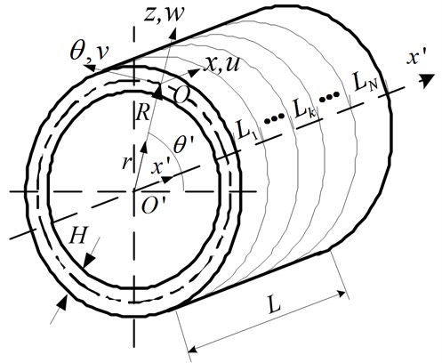
Figure 2 shows the nomenclature of a short thin cylindrical shell. The reference surface of the cylinder is taken at the middle surface where an orthogonal coordinate system () is fixed. The coordinates system () is the coordinates system () translate from origin along direction to one point of the middle surface. -axis and -axis are parallel and in the same direction. -axis and -axis are overlapping and in the same direction. -axis and -axis are overlapping. In the figure, is the radius, is the length, is the thickness, is the material density, is the Young's modulus and is the Poisson's ratio. The deformations of the cylindrical shell in the , and directions are denoted by , and , respectively. The short thin cylindrical shell is divided into sections along its length. The length of every section is , respectively.
Fig. 2The segmented mode of the thin-walled cylindrical shells
The bigger of , the more accurate of the result is, but it spends more time on achieving the result. Thus, the can’t be too large or too small. As shown in Table 2, the natural frequencies are very close when is 3, 4 and 5. Considering the time and accuracy, the is 3 in this paper.
Table 2The natural frequencies with different N (m=1, n=6)
1 | 2 | 3 | 4 | 5 | |
Natural frequencies | 14045.8 | 1377.44 | 1369.03 | 1369.02 | 1369.02 |
Based on the Kirchhoff theory, the shear and transversal shear are the following [13]:
Using the Love shell theory, the shell's equilibrium equations are expressed as vibration differential equation [14]:
The relationship of generalized force, corner and middle surface displacement are:
where , are the shell’s membrane stiffness, bending respectively.
The differential equations consist of Eq. (10)-(12), which contain 8 equations and 8 unknown variables. The unknown variables include 3 elastic displacement components, 1 rotation angle and 4 generalized force components. The unknown variables are expressed state vector which are defined as [15]:
Simplified Eq. (12) – Eq. (17) aiming at keeping only the state vector elements yields the following matrix equation:
The coefficient matrices of 8×8 order can be expressed in a general form as:
According to the geometric characteristics of thin-walled cylindrical shell, the middle surface generalized displacement and generalized force internal force of the short thin cylindrical shell along the direction are written as:
Substituting Eq. (21) into Eq. (19), the differential equation of modal function can be written as [16]:
where .
The coefficient matrices of 8×8 order can be expressed in a general form as:
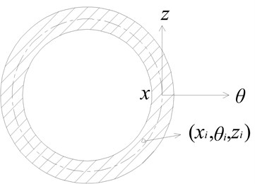
Suppose the cylinder is divided into sections, stress state of any point on the arbitrary cross-section of shell as shown in Figure 3.
Fig. 3Stress state of any point on the arbitrary cross-section
According to theory of solving differential equation, the general solution to state equation is the following:
where is the length of th shell segment, is transfer matrix and can be written as:
The modal function can be obtained by reusing transfer matrix and yields the following matrix equation:
where:
The coefficient matrices are obtained by Eq. (22). Using the Eq. (24) and Eq. (26), the transitive relation of the state vectors can be obtained. The transfer matrix is 8×8 matrix and can be written by calculating Eq. (27):
where are the transfer matrix coefficients.
3.2. Analytical method
The transfer matrixes are different on the different boundary conditions. The transfer matrixes are given as follows for the following boundary condition, and then the natural frequencies can be obtained.
a. Clamped-clamped
Set , ;
Set , .
Substitute Eq. (29) into Eq. (28), Eq. (29) are expressed as following:
The determinant of the coefficients of the matrix is zero:
The matrix is the function of natural frequencies. So the natural frequencies corresponding to modal are obtained.
b. Clamped-free
Set , ;
Set , ;
The determinant of the coefficients of the matrix is zero. So the natural frequencies corresponding to modal are obtained.
4. Numerical computation based on finite element method
In the classical vibration theory, the basic equation of dynamic problems based on finite element methods is presented as follows [17]:
where is the total mass matrix, is the total damping matrix, is the total stiffness matrix, is the total additional exciting force matrix, , and are the joint displacement, velocity and acceleration column matrixes respectively.
As the natural vibration frequency of structural system is calculated with the consideration that the free vibration is conducted under undamped conditions. The equation of the natural vibration frequency is expressed as:
The solutions can be presumed as the following types:
where is the order vector quantity, is the natural frequency.
The Eq. (33) is substituted into Eq. (34), and then generalized eigenvalue problems are obtained as follows:
According to the linear algebra theory, the necessary and sufficient conditions which allow Eq. (35) with untrivial solution are as follows:
where characteristic solutions can be obtained by solving these equations, such as among which stand for natural frequencies of system, and correspond to .
For every natural frequencies of structure, relative amplitudes of each node from one group can be concluded based on Eq. (35). Eigenvectors such as represent natural modes of vibration of structure. Their amplitudes can be set as follows:
Natural mode of vibration is orthogonal compared to matrix . Natural mode of vibration is defined as:
Then it can be obtained as follows:
The characters of characteristic solution can be also expressed as:
where and are the natural mode of vibration matrix and natural frequency matrix respectively.
5. The results of the three analytical methods
The natural frequencies of the static state of the cylindrical shell under clamped – free and clamped boundary conditions are calculated by the transfer matrix method, the beam function method and the finite element method, respectively, and make further verification of the natural frequencies. Table 3 shows the basic parameters of the thin-walled cylindrical shell.
Table 3The basic parameters of the thin-walled cylindrical shell
Young modulus (Pa) | Poisson's ratio | Density (kg/m3) | Length (mm) | Thickness (mm) | Inside radius (mm) | External radius (mm) | Material |
2.12×10¹¹ | 0.3 | 7850 | 95 | 2 | 142 | 144 | Structural steel |
Table 4The first 20 order natural frequencies in the clamped – free boundary conditions (Unit: Hz)
Order | 1 order | 2 order | 3 order | 4 order | 5 order |
Modal shape description | 1, 6 | 1, 5 | 1, 7 | 1, 4 | 1, 8 |
Transfer matrix | 1369 | 1424 | 1500 | 1701 | 1768 |
Beam function | 1717 | 1858 | 1734 | 2168 | 1893 |
Finite element | 1380 | 1450 | 1497 | 1739 | 1756 |
Order | 6 order | 7 order | 8 order | 9 order | 10 order |
Modal shape description | 1, 9 | 1, 3 | 1, 10 | 1, 11 | 1, 2 |
Transfer matrix | 2131 | 2230 | 2567 | 3062 | 3091 |
Beam function | 2174 | 2701 | 2552 | 3010 | 3636 |
Finite element | 2115 | 2274 | 2550 | 3048 | 3137 |
Order | 11 order | 12 order | 13 order | 14 order | 15 order |
Modal shape description | 1, 12 | 2, 7 | 2, 8 | 2, 6 | 2, 9 |
Transfer matrix | 3612 | 3611 | 3633 | 3752 | 3801 |
Beam function | 3536 | 3369 | 3411 | 3457 | 3572 |
Finite element | 3607 | 3686 | 3721 | 3818 | 3909 |
Order | 16 order | 17 order | 18 order | 19 order | 20 order |
Modal shape description | 2, 5 | 1, 13 | 2, 10 | 1, 1 | 2, 4 |
Transfer matrix | 4062 | 4215 | 4092 | 4437 | 4519 |
Beam function | 3683 | 4124 | 3841 | 4935 | 4062 |
Finite element | 4118 | 4223 | 4225 | 4476 | 4564 |
The natural frequencies of the cylindrical shell under clamped – free are calculated by the transfer matrix method, the beam function method and the finite element method respectively. Table 4 and Fig. 4 shows that the results of the transfer matrix method and the finite element method calculation are very close, the result of beam function method calculation is close to those of transfer matrix method and the finite element method calculation only at the place of 6th order, the 8th order, the 9th order and the 11th order, the frequencies of other orders are quite different.
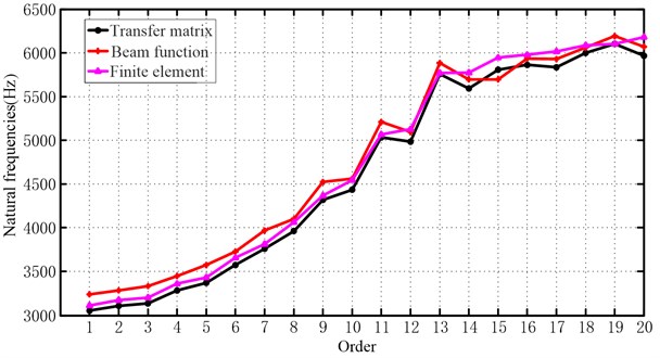
The natural frequencies of the cylindrical shell under both ends clamped boundary conditions are calculated by the transfer matrix method, the beam function method and the finite element method, respectively. Table 5 and Fig. 5 shows that the results of transfer matrix method and the finite element method calculation are very close, the result of beam function method calculation is close to those of transfer matrix method and the finite element method calculation only at the place of 8th order, the 10th order and the 12th order, the frequencies of other orders are quite different.
Fig. 4The frequencies comparison of the three methods in the clamped – free boundary condition
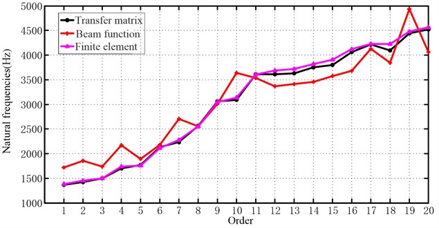
Table 5The first 20 order natural frequencies in the both ends clamped boundary condition (Unit: Hz)
Order | 1 order | 2 order | 3 order | 4 order | 5 order |
Modal shape description | 1, 7 | 1, 8 | 1, 6 | 1, 9 | 1, 5 |
Transfer matrix | 3051 | 3105 | 3136 | 3285 | 3369 |
Beam function | 3239 | 3282 | 3332 | 3449 | 3572 |
Finite element | 3115 | 3172 | 3198 | 3358 | 3428 |
Order | 6 order | 7 order | 8 order | 9 order | 10 order |
Modal shape description | 1, 10 | 1, 4 | 1, 11 | 1, 3 | 1, 12 |
Transfer matrix | 3576 | 3761 | 3964 | 4322 | 4435 |
Beam function | 3726 | 3967 | 4100 | 4522 | 4559 |
Finite element | 3657 | 3816 | 4059 | 4368 | 4547 |
Order | 11 order | 12 order | 13 order | 14 order | 15 order |
Modal shape description | 1, 2 | 1, 13 | 1, 1 | 1, 14 | 2, 7 |
Transfer matrix | 5034 | 4981 | 5759 | 5592 | 5804 |
Beam function | 5209 | 5094 | 5881 | 5696 | 5696 |
Finite element | 5066 | 5126 | 5770 | 5774 | 5943 |
Order | 16 order | 17 order | 18 order | 19 order | 20 order |
Modal shape description | 2, 6 | 2, 8 | 2, 5 | 1, 0 | 2, 9 |
Transfer matrix | 5862 | 5836 | 5996 | 6103 | 5963 |
Beam function | 5930 | 5929 | 6059 | 6189 | 6067 |
Finite element | 5974 | 6012 | 6086 | 6101 | 6179 |
Fig. 5The frequencies comparison of the three methods in the both ends clamped boundary condition
6. Experimental test and comparison
A method for identification the natural frequencies and the mode shape of cantilever circular cylindrical shells is presented, when striking it with a hammer. The hammering test system is shown in Fig. 6, they are impact measurement system consisting of modal hammer, polytec, LMS measurement system and a high-performance computer and so on.
Fig. 6Impact measurement system for modal of cantilever circular cylindrical shells
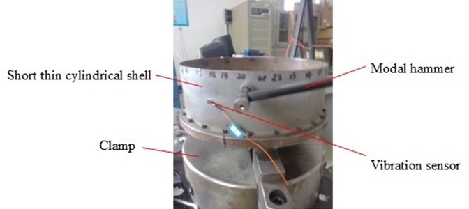
Table 6The results of experiments and finite element method
Order | Modal shape description | Experiment | Finite element | Difference (%) |
1 | 1,6 | 1065.3 | 1380 | 22.80 |
2 | 1,7 | 1310.6 | 1497 | 12.45 |
3 | 1,8 | 1627.9 | 1756 | 7.29 |
4 | 1,9 | 2005.6 | 2115 | 5.17 |
5 | 1,10 | 2436.1 | 2550 | 4.47 |
6 | 1,11 | 2916.0 | 3048 | 4.33 |
The natural characteristics are obtained by the way of multi-point excitation and a single point response, the drum is divided into five laps, and 36 points per circle, the sensors are fixed in the point (lap 10th point), an incentive hammer hammers sequentially 5×36 points.
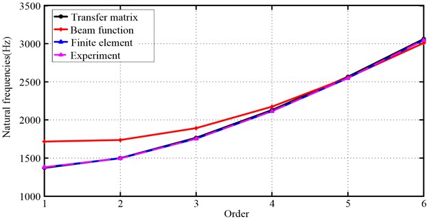
The results are shown in Table 6 and Fig. 7. The results of the transfer matrix method and the finite element method are close to that of experiments, while the results vary wildly between the transfer matrix method and the beam functions method, however the operation time of the beam functions method is short, and its calculation process is simple.
Fig. 7Three algorithms compared to experimental results
7. Conclusions
In this paper, analytical method (beam functions method), semi-analytical method (transfer matrix method) and numerical methods (finite element method) are presented to solve the natural characteristics of thin-walled cylindrical shell. The results in the clamped-free and clamped-clamped boundary conditions are focused on comparison. Furthermore, the experiments of the short thin cylindrical shell in the clamped-free boundary conditions are studied, which demonstrated that:
(1) Results of transfer matrix method and finite element method are basically similar, while great difference is obtained by beam functions method.
(2) Further studies by experiment have confirmed that the results obtained by transfer matrix method and finite element method are more accurate and efficient.
(3) Due to the influence of factors such as geometrical dimension, material parameters, machining accuracy and chucking ways, the biases between experimental results and calculation results is inevitable, but identical trends are observed during the study.
References
-
Wu Jialong. Elastic Mechanics. Higher Education Press, Beijing, 2001, (in Chinese).
-
C. B. Sharma, D. J. Johns. Free vibration of cantilever circular cylindrical shells – a comparative study. Journal of Sound and Vibration, Vol. 25, Issue 3, 1972, p. 433-449.
-
C. B. Sharma. Calculation of natural frequencies of fixed-free circular cylindrical shells. Journal of Sound and Vibration, Vol. 35, Issue 1, 1974, p. 55-76.
-
Young-Shin Lee, Young-Wann Kim. Effect of boundary conditions on natural frequencies for rotating composite cylindrical shells with orthogonal stiffeners. Advances in Engineering Software, Vol. 30, Issue 9-11, 1999, p. 649-655.
-
X. M. Zhang. Vibration analysis of cross-ply laminated composite cylindrical shells using the wave propagation approach. Applied Acoustics, Vol. 62, Issue 11, 2001, p. 1221-1228.
-
K. Y. Lam, C. T. Loy. Influence of boundary conditions for a thin laminated rotating cylindrical shell. Composite Structures, Vol. 41, Issue 3-4, 1998, p. 215-228.
-
Li Xuebin. A new approach for free vibration analysis of thin circular cylindrical shell. Journal of Sound and Vibration, Vol. 296, Issue 1-2, 2006, p. 91-98.
-
A. A. Jafari, S. M. R. Khalili, R. Azarafza. Transient dynamic response of composite circular cylindrical shells under radial impulse load and axial compressive loads. Thin-Walled Structures, Vol. 43, Issue 11, 2005, p 1763-1786.
-
Hamidzadeh H. R., Jazar R. N. Vibrations of Thick Cylindrical Structures. Springer, New York, 2010.
-
Hua Li, K. Y. Lam, T. Y. Ng. Rotating Shell Dynamics. Elsevier Science, 2005.
-
Zhang Yimin Mechanical Vibration. Tsinghua University Press, Beijing, 2007, p 192-193.
-
Yan Litang, Zhu Zigen, Li Qihan. High Speed Rotating Machinery Vibration. National Defence of Industry Press, Beijing, 1994.
-
Sun Shupeng. Dynamic Modeling and Analysis of Combined Revolving Thin-Walled Shells. Harbin Institute of Technology, Harbin, 2010.
-
Love E. H. A Treatise on the Mathematical Theory of Elasticity. Fourth Edition, Cambridge University Press, 1952.
-
Leon Y. Bahar. A state space approach to elasticity. Journal of the Franklin Institute, Vol. 299, Issue 1, 1975, p. 33-41.
-
Xiang Yu, Huang Yu-Ying, Lu Jing, et al. New matrix method for analyzing vibration and damping effect of sandwich circular cylindrical shell with viscoelastic core. Applied Mathematics and Mechanics, Vol. 29, Iusse 12, 2008, p. 1587-1600.
-
Yuan Anfu, Chen Jun. Application of ANSYS in model analysis. Manufacturing Technology & Machine Tool, Issue 8, 2007, p. 79-82.
About this article

This work is supported by National Science Foundation of China (51105064), National Program on Key Basic Research Project (2012CB026000), and Natural Science Foundation of Liaoning Province (201202056).
