Lamb wave temperature compensation method based on adaptive filter ADALINE network

2.1. Composite specimen and experimental step

In this paper, a stiffened carbon fiber composite panel of thickness 2 mm is adopted to study the temperature influence and the compensation method as shown in Fig. 1. PZTs (thickness 0.5 mm, diameter 8 mm, PIC255, PI L. P.) are mounted to the surface of the composite panel by using the epoxy adhesive 353ND (Epoxy Technology, Inc). The thickness of the adhesive layer is 0.08 mm approximately. 20 actuator-sensor channels are defined.

An environmental chamber Challenge 250 (Angelantoni Industrie SpA) which temperature controlling accuracy is ±0.3°C is adopted to simulate the temperature environment of PZTs. An integrated structural health monitoring system (ISS) [19] is adopted to fulfill the multi-channel scanning, frequency sweeping and Lamb wave signals acquiring of the 20 actuator-sensor channels constructed by the PZT sensors. In order to study the temperature influence of Lamb wave signals of different central frequencies, a five cycle sine burst is used as an excitation signal whose central frequency is swept from 50 kHz to 500 kHz with an interval of 50 kHz. The sampling rate is 10 MHz.

The temperature cycling in the experiment is performed in the following processes as illustrated in Fig. 2.

(1) Temperature pre-cycling. Temperature is continuously increased from 20 °C to 80 °C. Then it is continuously decreased to –40°C. Finally, temperature is continuously increased from –40°C to 20°C. The temperature pre-cycling is repeated for three times.

(2) Temperature cycling under health status. Temperature is continuously decreased from 20°C to –40°C with a cooling rate of 5°C/min and kept for 30 min at –40°C. And then, temperature is increased from –40°C to 80°C with a heating rate of 1 °C/min and kept for 30 min at 80°C. Then, temperature is decreased from 80°C to –40°C with a cooling rate of 1°C/min and kept for 30 min at –40°C. The Lamb wave signals are acquired from –40°C to 80°C and 80°C to –40°C of 2°C interval. Temperature cycling under health status is repeated for three times.

(3) Temperature cycling under damage status. A 100 g mass is bonded in the center of the area surrounded by PZT 5, PZT 6, PZT 8 and PZT 9 by 353ND to simulate damage. The temperature cycling is the same with temperature cycling under health status.

Through this experiment, Lamb wave signals under health and damage status at different temperatures and different central frequencies are acquired. As temperature cycling under health status is repeated for three times, six groups of Lamb wave health signals are acquired, including three in heating stage and three in cooling stage. In each temperature, there are six Lamb wave signals collected at different cycles. They are used as six samples to train and test the network in section 3.

Fig. 1Composite panel and PZTs placement

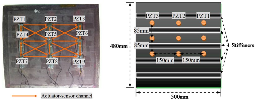
Fig. 2Temperature cycling illustration

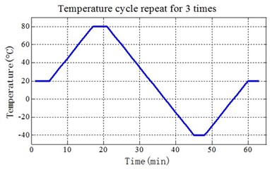
a) Temperature pre-recycling

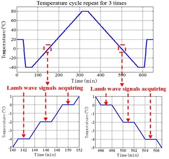
b) Temperature cycling under health or damage status

2.2. Temperature influence of Lamb wave signals

Fig. 3 gives out a waterfall plot of Lamb wave signals of actuator-sensor channel PZT1-PZT2 of different central frequencies at 20°C. The first wave packet in the signals is crosstalk signal introduced by the ISS. When the central frequency of excitation signal is low (50 kHz to 100 kHz), the amplitude of $S_0$ mode is low. But companying with the increasing of central frequency, the amplitude of $S_0$ mode becomes higher. In other words, only $A_0$ mode should be considered in low frequency. But $A_0$ and $S_0$ mode should be both considered in middle and high frequency.

Fig. 3Mode selection illustration

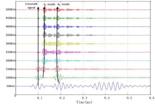
Fig. 4Temperature influence of Lamb wave signals of central frequency 50 kHz

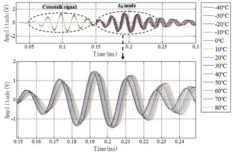
a) Lamb wave signals at different temperatures

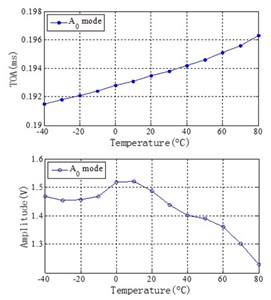
b) TOA and amplitude of $A_0$ mode versus temperature

Fig. 4 and 5 show the temperature influence of low and high central frequencies of Lamb wave signals, which come from actuator-sensor channel PZT1-PZT2. The temperature influences on time of arrival (TOA) and amplitude of Lamb wave signals are obvious. TOA has a good linear relationship versus temperature change for both $S_0$ and $A_0$ modes of different central frequencies. Temperature change will lead an approximately linear delay to the TOA of Lamb wave signals. Amplitude of $S_0$ and $A_0$ modes changed by temperature are more complicated and nonlinear.

Considering the linear relationship versus temperature of TOA and the nonlinear of amplitude, two parameters called as phase changing rate ($PCR$, unit rad/°C) and maximum amplitude variation ($MAV\text{,}$ unit %) are defined to quantify the temperature influence, respectively:

where $f_c$ is the central frequency of Lamb wave signals.

Fig. 5Temperature influence of Lamb wave signals of central frequency 400 kHz

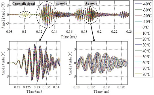
a) Lamb wave signals at different temperatures

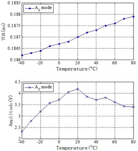
b) TOA and amplitude of $A_0$ mode versus temperature

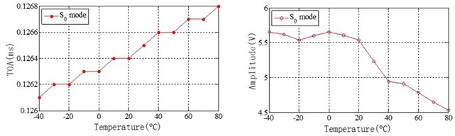
c) TOA and amplitude of $S_0$ mode versus temperature

Table 1 lists the two parameters of Lamb wave signals of different central frequencies. It shows that $A_0$ mode is more sensitive to temperature change than that of $S_0$ mode. PCR increase companying with the increasing of central frequencies. When the central frequency of excitation signal is low (50 kHz to 100 kHz), the amplitude of $S_0$ mode is very low and the $S_0$ mode is difficult to observe and analysis.

3.1. The general idea of the method

The procedure of temperature compensation method is shown in Fig. 6, including adaptive filter ADALINE network construction and temperature compensation with the network.

(1) Adaptive filter ADALINE network construction

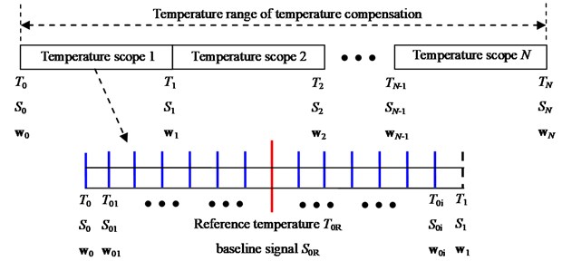
The whole temperature range from –40°C to 80°C is divided into many sub temperature scopes according to compensation standard and accuracy as shown in Fig. 7.

Taking the first temperature scope as an example, a reference temperature $T_{0R}$ is set to be the central temperature and the Lamb wave signal $S_{0R}$ at this temperature is set to be the baseline signal. Through the experiment of section 2, the Lamb wave signals at temperature $T_0,T_{01},\dots ,T_{0i}$ are acquired and set to be $S_0,S_{01},\dots ,S_{0i}$. $S_{0R}$ is considered to be input of adaptive filter ADALINE network and $S_0,S_{01},\dots ,S_{0i}$ are targets. After training the adaptive filter ADALINE network, a set of network parameters which are weights ${\mathbf{w}}_0,{\mathbf{w}}_{01},\dots ,{\mathbf{w}}_{0i}$ are acquired.

It should be emphasized that only one baseline signal and a set of weights of adaptive filter ADALINE network are needed to store in each temperature scope.

(2) Temperature compensation with the network

In damage monitoring, the environmental temperature and the Lamb wave signal at this temperature are acquired. According to the environmental temperature, the weights of the adaptive filter ADALINE network and the baseline signal are determined. Finally, the baseline signal of the temperature scope is input to the adaptive filter ADALINE network and the output is the compensated baseline signal at the environmental temperature.

Fig. 6Procedure of temperature compensation

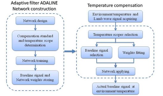
Fig. 7Temperature scopes illustration

3.2. Adaptive filter ADALINE network construction

The architecture of the adaptive filter ADALINE network which contains two layers referred as inputs and ADALINE are shown in Fig. 8. The layer of inputs is consisted of a tapped delay line. The input signal $f\left(t\right)$ enters from the left. At the output of the tapped delay line there is an $M$-dimensional vector, consisting of the input signal at the current time and the signals which are tapped delayed from $1$ to $M-1$ time steps. $M$ denotes the order of the tapped delay line. The output of the network can be presented as:

In the matrix from:

where $\mathbf{w}={\left[\begin{array}{cccc}{w}_1& w_2& \cdots & w_M\end{array}\right]}^T$, $\mathbf{z}={\left[\begin{array}{cccc}f\left(t\right)& f\left(t-1\right)& \cdots & f\left(t-M+1\right)\end{array}\right]}^T$.

Fig. 8Network architecture of adaptive filter ADALINE

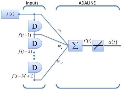
ADALINE (adaptive liner neural) network is shown in Fig. 8. It has the same basic structure as the perceptron network (one layer). The only difference is that it has a linear transfer.

In this paper, adaptive filter ADALINE network with 2 order tapped delay line ($M=$ 2) is selected to fulfill the temperature compensation task. In that case, a neuron with two weights and no bias is sufficient to implement the filter. Such a filter with 2 order tapped delay line can amplitude-change and phase-shift Lamb wave signal in the desired way. According to our research, $M$ is recommended set to be 2 for Lamb wave signal. Because ADALINE network with 2 orders tapped delay line is simple and easy to train. On the other side, when $M$ is set to be 3 or more than 3, the training results are not getting better and the weights become nonlinear to temperature.

The structure of adaptive filter ADALINE network is a classical uniform embedding with constant time lag equal to 1 which is capable to conduct amplitude-change and phase-shift Lamb wave signal in the desired way. Further study can be conducted on non-uniform embedding. The optimal time lags and optimal embedding dimensions for non-uniform embedding can be determined with the method proposed in [22].

In SHM applications, damage can be determined by evaluating maximum error of subtracted signal between monitoring signal and baseline signal. In that case, a normalized maximum error $Er$ is used to be the compensation standard and to validate the compensation results as shown in Eq. (5). It is a minimization criterion of the maximum amplitude to compare the similarity of the time domain signal:

where $a\left(t\right)$ is the output of the network, $f_T\left(t\right)$ is the target Lamb wave signal.

According to the Lamb wave signals acquired in health and damage status in section 2, the maximum error of their subtracted signals are –5.25 dB (PZT5-PZT9) and –29.78 dB (PZT1-PZT2). Combining the results from the research of Roy [14], temperature compensation standard is set as $Er<$ –25 dB. In this case, the temperature scope for $A_0$mode is set as 20 °C and it is 12 °C for $S_0$ mode.

Based on the compensation standard and the Lamb wave signals acquired in section 2, the network training for one temperature in one temperature scope can be performed. The goal of network training is to minimize the mean square error (MSE) of the target $f_T\left(t\right)$ and the output $a\left(t\right)$. The training function is the least mean square (LMS) algorithm [23].

The MSE of the network can be expressed as Eq. (6):

Here $E\left[\right]$ is expectation. This expression can be expanded and simplified to Eq. (7):

where $c=E\left[t^2\right],\mathbf{h}=E\left[t\mathbf{z}\right],\mathbf{R}=E\left[\mathbf{z}{\mathbf{z}}^T\right]$.

The gradient of MSE can be expressed as Eq. (8):

The LMS algorithm, with a constant learning rate $\alpha$, can be written as Eq. (9):

The learning rate can be set according to the following Eq. (10), (11) and (12):

where ${\lambda }_i$ are the eigenvalues of $\mathbf{R}$.

In this paper, the learning rate is set as be 0.0005.

For example, in order to obtain the weights at 20°C, the 4th temperature scope is selected and the reference temperature is set as 30°C. Thus, Lamb wave signal at 30°C is set to be the input of the network, while the signal at 20°C is the target of the network.

In section 2, six groups of Lamb wave health signals are acquired. Three samples of them are used for training the network, while the other three samples are used for testing the network with the compensation standard. The three samples of Lamb wave signals for training the network are set as input of the neural repeatedly until the weight matrix $\mathbf{w}$ converges. The weights of the network are an optimal solution for all the three samples after training.

The training convergence curve is shown in Fig. 9. After 30 thousand iteration steps, the weights is converges to (–3.57, 4.567) and the $MES$ converges to 1.6×10^-3. After training, the normalized maximum errors between output and target is –28 dB which is less than –25 dB and meet the compensation standard. Through the process mentioned above, the weights of adaptive filter ADALINE network for one temperature in one temperature scope are obtained.

Fig. 9Convergence curve of network training of one temperature in one temperature scope

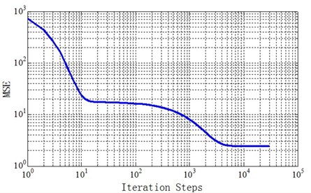
Fig. 10Weights changed with temperature

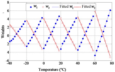
The weights of the network at the other temperature in each temperature scope can be obtained in the same way. The network architecture for each temperature is the same, while the weights of the network are altered according to the monitoring temperature.

As the temperature acquired by a temperature sensor is not always integers, there is great importance to fit the weights to improve accuracy. As shown the solid blue line in Fig. 10, the weights are linear to temperature at each temperature scope. Thus, the least square linear fit is implemented to fit the weights which are shown the dotted red line in Fig. 10.

Once a set of weights are obtained and their performance meet the compensation standard, they can be adopted in adaptive filter ADALINE network to temperature compensation which is based on Eq. (4).

4.1. Temperature compensation of ${\mathit{A}}_0$ mode

According to the compensation standards and requirements, temperature compensation scope for $A_0$ mode is determined as 20 °C. Lamb wave signals of six reference temperatures (which are –30 °C, –10 °C, 10 °C, 30 °C, 50 °C, 70 °C) are acquired and stored in the baseline signal database. The weights are trained and fitted to obtain the weights at each temperature.

Then according to the environmental temperature, the weights of the adaptive filter ADALINE network and the baseline signal are determined. Finally, the baseline signal of the temperature scope is input to the adaptive filter ADALINE network and the output is the compensated baseline signal at the environmental temperature.

Fig. 11Compensate baseline signal (30°C) to target signal (20°C)

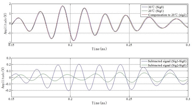
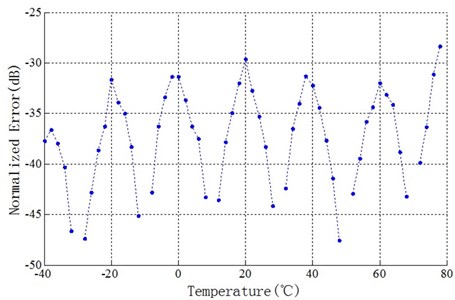
Fig. 12A0mode compensation result

For example, the environment temperature is at 20°C. In that case, the fourth temperature scope is selected and the reference temperature for this scope is 30°C. Thus, baseline signal at 30 °C is selected as the input of the network. On the other hand, the network weights for 20°C are selected from the set of weights trained in section 3. After applying the network, the output of the network is the compensated signal at 20°C, as shown in Fig. 11. The figure illustrates that the amplitude of subtracted signal between Lamb wave signals obtained 20°C and 30°C is up to 0.2 V, while after compensation it is less than 0.07 V (normalized maximum error is –28 dB) which meet the compensation standard.

For compensating the signal at other temperature, the same algorithm can be used. The compensation results are verified at each temperature as illustrated in Fig. 12. In stiffened composite panel, temperature various from –40°C to 80°C, temperature compensation scope of baseline signal is set as 20°C for $A_0$ mode. After compensation, the normalized maximum errors are less than –25 dB at each temperature.

4.2. Temperature compensation of ${\mathit{S}}_0$ mode

According to the compensation standards and requirements, temperature compensation scope for $S_0$ mode is determined as 12°C. Lamb wave signals of ten reference temperatures (which are –34°C, –22°C, –10°C, 2°C, 14°C, 26°C, 38°C, 50°C, 62°C, 74°C) are acquired and stored in the baseline signal database. The weights are trained and fitted to obtain the weights at each temperature.

Fig. 13Compensate baseline signal (26°C) to target signal (20°C)

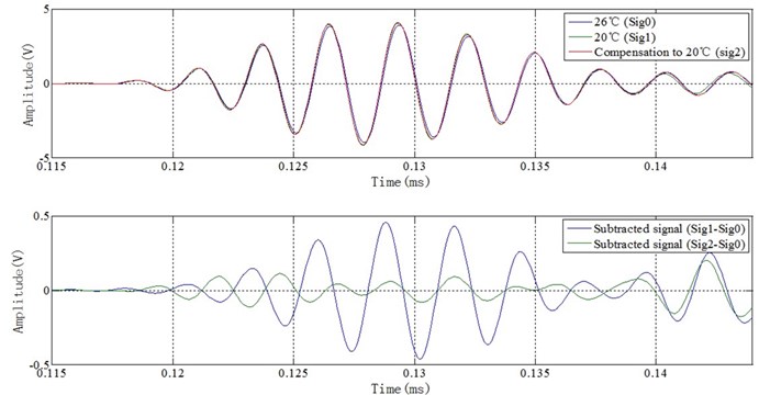
Fig. 14S0 mode compensation result

The method compensate for $S_0$ mode is the same as $A_0$ mode. For example, the environment temperature is at 20°C. In that case, the sixth temperature scope is selected and the reference temperature for this scope is 26°C. Thus, the baseline signal at 26°C is selected as the input of the network. On the other hand, the network weights for 20°C are selected from the set of weights trained in section 3. After applying the network, the output of the network is the compensated signal at 20°C, as shown in Fig. 13.

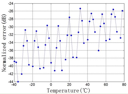
For compensating the signal at other temperature, the same algorithm can be used. The compensation results are verified at each temperature as illustrated in Fig. 14. In stiffened composite panel, temperature various from –40°C to 80°C, temperature compensation scope of baseline signal is set as 12°C for $S_0$ mode. After compensation, the normalized maximum errors are less than –25 dB at each temperature.

4.3. Damage imaging combination with temperature compensation

The delay-and-sum imaging algorithm [21, 24] is applied in this section to determined the health status of the monitoring area. The algorithm compares the signal of the structure at health and damage status and determines the damage location. The actual damage is located in the center of the area surrounded by PZT 5, PZT 6, PZT 8 and PZT 9 and coordinate of the damage is (–75 mm, –42.5 mm).

With the signals recorded in section 2, four typical conditions for engineering application are demonstrated in the following to validate compensation results.

(1) Temperature effect cause false alarms

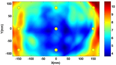
When the temperature changes, even the structure are not damaged, the algorithm shows false alarms. For example, the health signal at 20°C is set to be Health Signal of the imaging algorithm, while the health signal at 30°C is set to be Damage Signal. The imaging result shows a false damage in (160 mm, 104 mm) as demonstrated in Fig. 15(a). The point with the pixel peak value of the imaging result is often regarded as the damage location.

(2) Image result without compensation

Another condition is that under the influence of temperature, even the structure is damaged, the algorithm cannot determine the right location of damage. An example is given: the health signal at 20°C is set to be Health Signal of the imaging algorithm, while the damage signal at 30°C is set to be Damage Signal. The imaging result shows damage located in (172 mm, –15 mm) as demonstrated in Fig. 15(b). The damage information is concealed by temperature effect. The result shows that it is very important to conduct temperature compensation.

(3) Image result with compensation

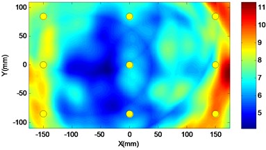
In this condition, the health signal at baseline temperature is compensated to health signal at the target temperature. For example, the ADALINE network is applied to compensate the health signal at 20°C to the compensational health signal at 30°C. The compensational health signal at 30°C is set to be Health Signal of the imaging algorithm, while the damage signal at 30°C is set to be Damage Signal. The imaging result shows a damage in (–70 mm, –44 mm) as demonstrated in Fig. 15(c). The result shows that after compensation, great accuracy is acquired with an error of 5.2 mm.

(4) Traditional damage detection

In the last condition, the health signal is recorded at the target temperature and is used in damage imaging with the damage signal at target temperature. The health signal at 30°C is set to be Health Signal of the imaging algorithm, while the damage signal at 30°C is set to be Damage Signal. The imaging result shows a damage in (–70 mm, –43 mm) as demonstrated in Fig. 15(d). The result shows that the damage image result is the same as the compensated result.

Generally speaking, temperature effects will cause false alarms and conceal the damage information. After compensation, great accuracy is acquired with an error of 5.2 mm. The proposed temperature compensation method is effective and has been verified by the damage detection.

Fig. 15Damage imaging results

a) Temperature effects cause false alarms

b) Image result without compensation

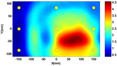
c) Image result with compensation

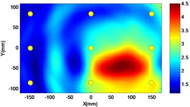
d) Image result at 30 °C