Ride comfort analysis of a nonlinear vehicle excited by the consecutive speed-control humps

Liang, Shan; Sun, Yongsheng; Zhu, Qin; Yang, Zhiyong; Zeng, Cheng

Journal of Vibroengineering

Browse Journal

Submit article

Published: 31 December 2013

Check for updates

Ride comfort analysis of a nonlinear vehicle excited by the consecutive speed-control humps

Shan Liang¹

Yongsheng Sun²

Qin Zhu³

Zhiyong Yang⁴

Cheng Zeng⁵

^{1, 2, 4, 5}College of Automation, Chongqing Univers, Chongqing 400044, China

³Department of Mechanical Engineering, Oyama National College of Technology, Oyama 323-0806, Japan

⁴College of Information and Engineering, Chongqing Vocational Institute of Engineering, Chongqing 400037, China

Corresponding Author:

Shan Liang

Cite the article Download PDF

Downloads 1559

WoS Core Citations 6

Abstract

The consecutive speed-control humps (SCHs) possess the function of controlling speed forcibly, but cause violent vibration of a vehicle inevitably. This paper tries to further explore the inherent link among parameters of the SCHs, velocity and vehicle vibration. A 4-DOF nonlinear half-vehicle model with nonlinear springs and nonlinear dampers is established. The consecutive SCHs-speed coupling excitation function is presented by combination of trapezoidal and sine wave of constant amplitude and variable frequency. The nonlinear dynamics of half-vehicle model is investigated by numerical simulation. It reveals that various forms of vibrations, such as periodic, quasi-periodic and chaotic vibrations, could appear in the system with the change of the velocity. Further it is found that quasi-periodic motions will affect vehicle ride comfort most and can be avoided by changing parameters of the consecutive SCHs. Results are conductive to deep understanding of nonlinear vibration in vehicle and rational design of the consecutive SCHs.

1. Introduction

The speed-control hump (SCH) which is installed on highway is currently widely used as one of the compulsive speed control facilities. In general, the consecutive SCHs are local elevations of residential road surface of limited height, which are placed in series at hundreds or thousands of meters with a fixed interval. When the automobile passes over the consecutive SCHs at a certain velocity, the impact from the uneven road surface will inevitably bring to the vehicle unwanted vibrations and noise. Prolonged exposure to repeated vibrations and impacts of whole-body nature when vehicle travels on uneven road has been associated to occupational health disorders [1]. Therefore the effect of the consecutive SCHs on vehicle vibrations, and in particular on the ride comfort, is still needed to be further studied [2-5].

Since the automobile is a kind of highly nonlinear system, the vibrations caused by road surface will appear in nonlinear characters, such as chaos and bifurcation. To investigate nonlinear response of vehicle model excited by road surface, some productive works have been done by scholars. In these studies researchers often rely on the quarter-car model for studying heave motion as this model is the simplest to analyze and yet can reasonably predict the response of a system [6-8]. However the actual vehicle is a more complex nonlinear system than a quarter-car model system. The vehicle speed, pitch motion, roll motion and the impact of front and rear wheels are also important to the dynamics of actual vehicle. Zhu et al. [9, 10] have investigated the possibilities of chaotic vibrations which existed in half-car and full-car models under sine wave excitations. However the influence of vehicle speed on vehicle dynamics and how the nonlinear vibrations affect the vehicle ride comfort have rarely been investigated in the current studies.

In this paper the nonlinear vibration behaviours of the 4-DOF half-vehicle model with nonlinear springs and damping elements through the excitations from the consecutive SCHs are investigated. The study begins by establishing a combined consecutive SCHs-speed dynamic excitation function and the nonlinear 4-DOF half-vehicle mechanical model. Then the numerical simulation is carried out for investigating the dynamic responses of the simplified vehicle system. Results show that the complex behaviours, such as quasi-periodic and chaotic vibrations, may exist in the system. Quasi-periodic motion deteriorates vehicle ride comfort significantly, which can be avoided by changing the parameters of the consecutive SCHs.

2. The excitation model of the consecutive SCHs

In general, there are some shapes of the consecutive SCHs in the special sections on the highway. When a vehicle passes over a series of SCHs with a certain speed, the trajectory of the vehicle can be approximately considered as the periodic trapezoidal wave [11]. The consecutive speed-control humps and its model of trapezoidal excitation are illustrated as in Fig. 1a and Fig. 1b, respectively.

Fig. 1Consecutive SCHs excitation

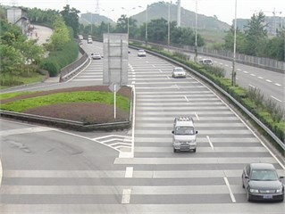
a) Consecutive SCHs road

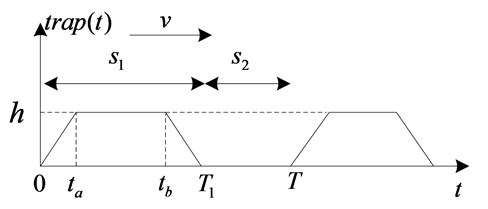
b) Road profile of the SCH surface

In Fig. 1b, $h$ is the amplitude of consecutive SCHs excitation, $s_{1}$ and $s_{2}$ are the width of a hump and the gap between two adjacent humps, $T_{1}$ is the time to pass a hump for a vehicle, $[T_{1}, T]$ is the time to pass the gap between two adjacent humps. If we take the roughness of the road surface into account, then a sinusoidal wave can be viewed as the intrinsic excitation of the road surface. The combination of a sinusoidal wave and a trapezoidal wave is used to describe the excitation generated by consecutive speed-control hump area on highway. Thus, the consecutive speed control humps can be approximated as:

1

x_{r} (t) = t r a p (t) + A \cdot s i n (2 π f_{2} t),

where $A$ is the amplitude of sinusoidal excitation, $f_{2}$ is the intrinsic excitation frequency caused by road surface roughness, $t r a p (t)$ stands for the trapezoidal wave, which can be expressed as follows:

2

t r a p (t) = \{\begin{array}{l} \frac{h}{t_{a}} \times t, & t \leq t_{a}, \\ h, & t_{a} < t \leq t_{b}, \\ \frac{h}{T_{1} - t_{b}} \times (T_{1} - t), & t_{b} < t \leq T_{1}, \\ 0, & T_{1} < t < T, \end{array}

where $T_{1} = T / 2$ , $t_{a} = T_{1} / 4$ and $t_{b} = T_{1} - T_{1} / 4$ and $T$ is the period of consecutive SCHs excitation. Define $f_{1}$ is the frequency of consecutive SCHs excitation, then:

3

f_{1} = \frac{1}{T} = \frac{v}{s_{1} + s_{2}} .

Obviously $f_{1} < f_{2}$ . Assume the following equation holds:

4

f_{2} = σ \cdot f_{1} = \frac{σ}{T} = \frac{σ \cdot v}{s_{1} + s_{2}},

where $σ$ is defined as the ratio of $f_{1}$ and $f_{2}$ , $s_{1}$ and $s_{2}$ are width of a hump and the gap between two adjacent humps, respectively.

For half-vehicle model, the excitations to the front and rear tire are defined respectively as:

5

\{\begin{array}{l} x_{f d} (t) = t r a p (t) + A \cdot s i n (2 π f_{2} t), \\ x_{r d} (t) = x_{f d} (t + Δ t) = t r a p (t + Δ t) + A \cdot s i n [2 π f_{2} (t + Δ t)], \end{array}

where $Δ t$ is the time delay between the forcing functions $x_{f d}$ and $x_{r d}$ , which can be calculated by the vehicle speed and the distance between front and rear wheels.

3. Four-DOF suspension model

Assuming the vehicle has a bilaterally symmetric structure, it is reasonable to simplify the vehicle as a four-DOF suspension model as in Fig. 2 [9].

Fig. 2Nonlinear four-DOF half-vehicle model

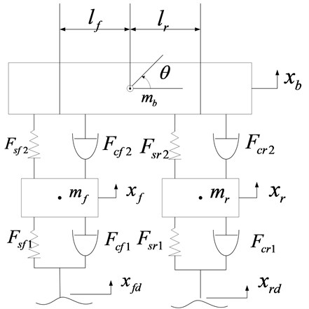
The notations used in the model (Fig. 2) are defined as following:

$m_{b}$ : vehicle body mass; $m_{f}$ , $m_{r}$ : front and rear unsprung masses, respectively; $θ$ : angular displacement of vehicle body; $x_{b}$ : vertical displacement of vehicle body; $x_{f}$ : heave displacement of $m_{f}$ ; $x_{r}$ : heave displacement of $m_{r}$ ; $x_{f d}$ , $x_{r d}$ : excitations to the front and rear tires; $F_{s f 1}$ , $F_{s r 1}$ : front and rear nonlinear tire spring forces; $F_{s f 2}$ , $F_{s r 2}$ : front and rear nonlinear suspension spring forces; $F_{c f 1}$ , $F_{c r 1}$ : front and rear nonlinear tire damper forces; $F_{c f 2}$ , $F_{c r 2}$ : front and rear nonlinear suspension damper forces. By analyzing the mechanical model, the equation of $x_{r d}$ , the equations of motion can be expressed as:

6

\{\begin{array}{l} m_{b} {\ddot{x}}_{b} = - F_{s f 2} - F_{c f 2} - F_{s r 2} - F_{c r 2} - m_{b} g, \\ J \ddot{θ} = (F_{s f 2} + F_{c f 2}) l_{f} c o s θ - (F_{s r 2} + F_{c r 2}) l_{r} c o s θ, \\ m_{f} {\ddot{x}}_{f} = F_{s f 2} + F_{c f 2} - F_{s f 1} - F_{c f 1} - m_{f} g, \\ m_{r} {\ddot{x}}_{r} = F_{s r 2} + F_{c r 2} - F_{s r 1} - F_{c r 1} - m_{r} g, \end{array}

where $J$ is vehicle body inertia. The spring forces $F_{s i j}$ are assumed to have the following characteristics [12, 13]:

7

F_{s i j} = k_{i j} s g n (Δ_{i j}) {|Δ_{i j}|}^{n_{i j}}, (i = f, r; j = 1, 2),

where $i = f, r$ denotes front or rear wheel, $j = 1, 2$ denotes suspension or tire, the definitions of $i$ and $j$ are suitable for other formulas in the paper, $k_{i j}$ is the equivalent stiffness, $Δ_{i j}$ is the deformation of the spring, $n$ is an exponent suspension spring. Therefore $Δ_{f 1}$ , $Δ_{f 2}$ , $Δ_{r 1}$ and $Δ_{r 2}$ can be given as follows:

$Δ_{f 1} = x_{f} - Δ_{s f 1} - x_{f d}$ , $Δ_{f 2} = x_{b} - Δ_{s f 2} - x_{f} - l_{f} s i n θ$ ,

$Δ_{r 1} = x_{r} - Δ_{s r 1} - x_{r d}$ , $Δ_{r 2} = x_{b} - Δ_{s r 2} - x_{r} + l_{r} s i n θ$ .

The dampers of tires and springs are assumed to be viscous, so the characteristics of damping force can be expressed as:

8

F_{c i j} = c_{i j} Δ {\dot{x}}_{i j}, (i = f, r; j = 1, 2),

where $F_{c i j}$ is the damping force and $Δ {\dot{x}}_{i j}$ is the relative velocity of the extremes of the damper. The damping coefficients are defined as:

9

c_{i j} = \{\begin{array}{l} c_{i j u}, & Δ {\dot{x}}_{i j} \geq 0, \\ c_{i j d}, & Δ {\dot{x}}_{i j} < 0, \end{array} (i = f, r; j = 1, 2),

where $c_{i j u}$ and $c_{i j d}$ are the damping coefficients for tension and compression, respectively.

Letting $x_{1} = x_{b}$ , $x_{2} = {\dot{x}}_{b}$ , $x_{3} = θ$ , $x_{4} = \dot{θ}$ , $x_{5} = x_{f}$ , $x_{6} = {\dot{x}}_{f}$ , $x_{7} = x_{r}$ , $x_{8} = {\dot{x}}_{r}$ , the state equations of the 4-DOF suspension system can be expressed as:

10

\{\begin{array}{l} {\dot{x}}_{1} = x_{2}, \\ {\dot{x}}_{2} = - \frac{1}{m_{b}} (F_{s f 2} + F_{c f 2} + F_{s r 2} + F_{c r 2}) - g, \\ {\dot{x}}_{3} = x_{4}, \\ {\dot{x}}_{4} = \frac{c o s θ}{J} [(F_{s f 2} + F_{c f 2}) l_{f} - (F_{s r 2} + F_{c r 2}) l_{r}], \\ {\dot{x}}_{5} = x_{6}, \\ {\dot{x}}_{6} = \frac{1}{m_{f}} (F_{s f 2} + F_{c f 2} - F_{s f 1} - F_{c f 1}) - g, \\ {\dot{x}}_{7} = x_{8}, \\ {\dot{x}}_{8} = \frac{1}{m_{r}} (F_{s r 2} + F_{c r 2} - F_{s r 1} - F_{c r 1}) - g, \end{array}

where $m_{b f}$ and $m_{b r}$ are the partial masses for front and rear axles of the system, and:

11

m_{b f} = \frac{m_{b} l_{r}}{l_{f} + l_{r}}, m_{b r} = \frac{m_{b} l_{f}}{l_{f} + l_{r}} .

When the suspension system is in the relatively static state of equilibrium, there are no external excitations and relative speed, then the following equations are valid:

12

\{\begin{array}{l} F_{s f 1} = k_{f 1} s g n (Δ_{s f 1}) {|Δ_{s f 1}|}^{n_{f 1}} = (m_{b f} + m_{f}) g, \\ F_{s r 1} = k_{r 1} s g n (Δ_{s r 1}) {|Δ_{s r 1}|}^{n_{r 1}} = (m_{b r} + m_{r}) g, \\ F_{s f 2} = k_{f 2} s g n (Δ_{s f 2}) {|Δ_{s f 2}|}^{n_{f 2}} = m_{b f} g, \\ F_{s r 2} = k_{r 2} s g n (Δ_{s r 2}) {|Δ_{s r 2}|}^{n_{r 2}} = m_{b r} g . \end{array}

Therefore, the static deformations $Δ_{s f 1}$ , $Δ_{s f 2}$ , $Δ_{s r 1}$ and $Δ_{s r 2}$ can be evaluated by (12).

Assume that $δ_{x b}$ is the initial heave displacement of $m_{b}$ and $Δ_{θ}$ , then the initial angular displacement $δ_{x b}$ and $Δ_{θ}$ can be calculated as:

13

δ_{x b} = \frac{l_{f} Δ_{s r 2} + l_{r} Δ_{s f 2}}{l_{f} + l_{r}}, Δ_{θ} = a r c s i n (\frac{Δ_{s f 2} - Δ_{s r 2}}{l_{f} + l_{r}}) .

Therefore the initial condition of state variables can be set as:

14

[x_{1}, x_{2}, x_{3}, x_{4}, x_{5}, x_{6}, x_{7}, x_{8}] = [- δ_{x b}, 0, Δ_{θ}, 0, - Δ_{s f 2}, 0, - Δ_{s r 2}, 0] .

4. Numerical analysis

Owing to the nonlinearity of the system (10), the dynamic response of the vehicle model can be studied numerically by the fourth-order Runge-Kutta algorithm provided by MATALB.

Table 1 shows parameters for numerical simulation as an example [9].

Table 1Parameters for numerical simulation

Parameter	Value	Parameter	Value	Parameter	Value
$m_{b}$	1180.0 kg	$J$	633.615 kg·m²	$c_{f 2 u}$ , $c_{r 2 u}$	500 N·m/s
$m_{f}$	50.0 kg	$g$	9.81 N/kg	$c_{f 2 d}$ , $c_{r 2 d}$	359.7 N·m/s
$m_{r}$	45.0 kg	$l_{f}$	1.123 m	$c_{f 1 u}$ , $c_{r 1 u}$	10 N·m/s
$k_{f 2}$	36952.0 N/m	$l_{r}$	1.377 m	$c_{f 1 u}$ , $c_{r 1 u}$	10 N·m/s
$k_{r 2}$	30130.0 N/m	$n_{f 2}$ , $n_{r 2}$	1.5	$h$	0.02 m
$k_{f 1}$ , $k_{r 1}$	14000.0 N/m	$n_{f 1}$ , $n_{r 1}$	1.25	$s_{1}$ , $s_{2}$	0.5 m
$A$	0.0015 m	$σ$	10

4.1. Nonlinear dynamics analysis of the system

In general, for nonlinear dynamics analysis of a system, the transient process and stationary process are two issues of crucial importance. However the kinetic characteristics of a mechanical system could be evident only when the system tends to be stable. In order to investigate the nonlinear dynamics of the studied system, in this paper the system kinetic characteristics are explored by investigating dynamics of stationary process and the corresponding speed ranges of the different kinetic performances are obtained through speed bifurcation diagrams, phase portraits, Poincaré maps and power spectrums.

In this section speed bifurcation diagrams are first introduced for analyzing the dynamics of the vehicle suspension system, which are obtained by plotting the Poincaré points of the state variables ( $x_{b}$ and $θ$ etc. in this paper) at different velocities. For a certain speed, the complexity of the system is usually proportional to the number of Poincaré points. Single-point indicates periodic motion and multi-point may mean period-doubling, quasi-periodic or chaotic motion. Speed bifurcation diagrams could roughly represent the system kinetic characteristics and intuitively investigate the effects of speed on the dynamics of the system.

Fig. 3Speed bifurcation diagram of xb

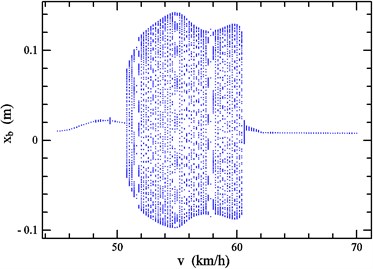
Fig. 4Speed bifurcation diagram of θ

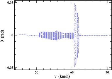
Fig. 3-4 respectively represent the speed bifurcation diagrams of $x_{b}$ and $θ$ when $v$ varies in 45.0 km/h ~ 70.0 km/h, where simulation time: $t =$ 20 s, simulation step: $Δ v =$ 0.2 km/h. As can be shown in the Figures, there are visible differences in the vibration performance when the speed is in different scopes. Based on these, the considered speed range can be broadly classified into three regions: region A (45.0 km/h ~ 50.6 km/h), region B (50.6 km/h ~ 62.0 km/h), region C (62.0 km/h ~ 70.0 km/h). It’s obvious that the system kinetic characteristics are similar when $v$ is in a same region. To investigate specific kinetic characteristics in the three regions, the phase portrait, Poincaré map and power spectrum at $v =$ 47.6 km/h, 54.0 km/h, 64.0 km/h are investigated in Fig. 5-7, respectively.

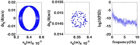
As shown in Fig. 5-7, the characteristics of vertical vibration of vehicle body are separately periodic, quasi-periodic or chaotic when speeds are 47.6 km/h, 54.0 km/h or 64.0 km/h, which implies that the system performs stable periodic motion in region A; when $v$ varies in region B, the system appears in the quasi-period motion; as $v$ increases to region C, the chaotic motion takes place in the system.

Fig. 5Periodic motion (v= 47.6 km/h)

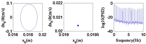
Fig. 6Quasi-periodic motion (v= 54.0 km/h)

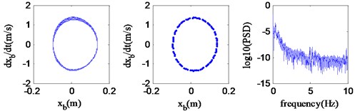
Fig. 7Chaotic motion (v= 64.0 km/h)

4.2. Ride comfort analysis of vehicle model

By the analysis above, the nonlinear vibrations of the vehicle may present periodic, quasi-periodic and chaotic features when system is in the stable regimes. But in fact the time to pass over the consecutive SCHs is relatively short for a real car. Therefore, in order to analyse vehicle model under the excitation of the consecutive SCHs, transient process is also important. In this paper vehicle Vibration Amplitude (VA) and Vibration Strength (VS) are introduced for ride comfort analysis of vehicle model.

Fig. 8Time-domain responses of vibration amplitude (blue: v= 47.6 km/h, red: v= 54.0 km/h, green: v= 64.0 km/h)

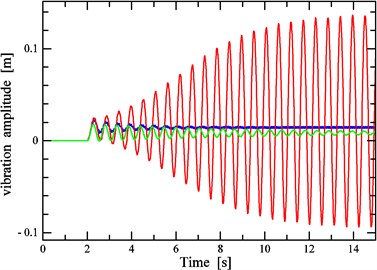
Fig. 9Time-domain responses of vibration strength (blue: v= 47.6 km/h, red: v= 54.0 km/h, green: v= 64.0 km/h)

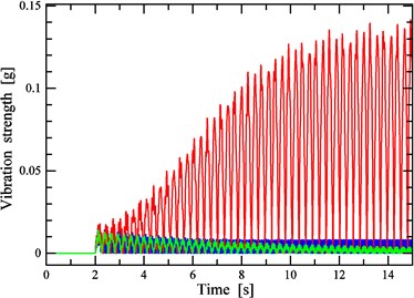
Fig. 8 and Fig. 9 separately represent the time-domain responses of the VA and VS of the vehicle model under the consecutive SCHs excitation. In both of them it is supposed that the vehicle begins to pass into the consecutive SCHs zone when Time $=$ 2 s, and the three kinds of lines with different colors are the time-domain curves of the vehicle vibrations when the vehicle is at 47.6 km/h, 54.0 km/h and 64.0 km/h, which represent nonlinear vibrations in region A, B, and C, respectively.

As shown in Fig. 8 and Fig. 9, there are significant differences in the behaviours of the system when the speed is in region A, B and C. In region B, the VA and VS of the system diverges dramatically since the vehicle begins to pass into the consecutive SCHs zone and keeps quasi-periodic motions at high levels when stable, which means ride comfort gets worse sharply when passing over the consecutive SCHs. In the meantime, the VA and VS values of the system, speeds of which belong to region A or C, are convergent at the transient process and fluctuate at relatively low levels, which means that the effects of extra vibrations caused by consecutive SCHs on ride comfort are not obvious.

4.3. Relations between the consecutive SCH and vehicle ride comfort

From the analysis above, it is clear that vehicle model has a bad ride comfort when the system meets the conditions of quasi-periodic motions. For the sake of safety, vehicles are required to travel over a speed hump road in a restricted range of speed. Therefore it’s a feasible way to design the appropriate parameters of consecutive SCH and avoid such scope of speed becoming to the quasi-period region. Table 2 represents the relations between the parameters of the consecutive SCHs and the range of speed in which results in vehicle excessive vibrations. $s$ is defined as the width of SCH, $s = s_{1} + s_{2}$ , $δ$ is defined as the duty ratio of humps, $δ / 100 = s_{1} / (s_{1} + s_{2})$ .

As shown in Table 2, the values of speed range become larger when the width of SCH increases. However, the values decrease with the duty ratio of humps increasing. It means one can obtain a good ride comfort by changing $s$ or $δ$ (or the both ones) so that the vehicle which is traveling in the restricted speed will not cause excessive vibrations.

Table 2Relations between the parameters of consecutive SCH and vehicle speed of great vibrations

$δ = 50$ , $s$ / (m)	The speed range / (km/h)	$s_{1} =$ 0.05 m, $δ$	The speed range / (km/h)
0.8	38.7 $< v <$ 49.8	45	56.0 $< v <$ 66.7
1	50.6 $< v <$ 62.0	50	50.6 $< v <$ 62.0
1.2	60.3 $< v <$ 73.2	55	46.4 $< v <$ 55.3

5. Conclusions

In the paper the nonlinear dynamics of a 4-DOF vehicle suspension model under the consecutive SCHs excitation is studied through numerical simulation. Results show that the periodic motion, quasi-periodic motion and chaotic motion will occur in the system when the vehicle travels over the consecutive SCHs with the increase of vehicle velocity. Vehicle ride comfort becomes bad when quasi-periodic response occurs in the system and it can be improved effectively by changing the parameters of consecutive SCHs.

Although the mechanical model of vehicle and the consecutive SCHs are only simplified ones and the parameters used do not agree precisely with the practical data for actual vehicles, the results may still be useful in the design of a ground vehicle and the cognition of dynamics response of vehicle when driving in a special pavement structure.

References

Bengt-Olov Wikström, et al. Health effects of longterm occupational exposure to whole-body vibration: a review. International Journal of Industrial Ergonomics, Vol. 14, 1994, p. 273-292.

Search CrossRef
A. Sezgin, Yz. Arslan. Analysis of the vertical vibration effects on ride comfort of vehicle driver. Journal of Vibroengineering, Vol. 14, 2012, p. 559-571.

Search CrossRef
Zifan Fang, et al. Mechatronics in Japanese rail vehicles: active and semi-active suspensions. Control Engineering Practice, Vol. 10, 2011, p. 428-437.

Search CrossRef
Wei-Yen Wang, et al. Hierarchical fuzzy-neural control of anti-lock braking system and active suspension in a vehicle. Automatica, Vol. 48, 2012, p. 1698-1706.

Search CrossRef
G. Priyandoko, M. Mailah, H. Jamaluddin. Vehicle active suspension system using skyhook adaptive neuro active force control. Mechanical Systems and Signal Processing, Vol. 23, 2009, p. 855-868.

Search CrossRef
S. Liang, C. Li, Q. Zhu, Q. Xiong. The influence of parameters of consecutive speed control humps on the chaotic vibration of a 2-DOF nonlinear vehicle model. Journal of Vibroengineering, Vol. 13, 2011, p. 406-413.

Search CrossRef
S. Li, S. Yang, W. Guo. Investigation on chaotic motion in hysteretic non-linear suspension system with multi-frequency excitations. Mechanics Research Communications, Vol. 31, 2004, p. 229-236.

Search CrossRef
Utz Von Wagner. On non-linear stochastic dynamics of quarter car models. Int. J. Non-Linear Mech., Vol. 39, 2004, p. 753-765.

Search CrossRef
Q. Zhu, M. Ishitobi. Chaos and bifurcations in a nonlinear vehicle model. Journal of Sound and Vibration, Vol. 275, 2004, p. 1136-1146.

Search CrossRef
Q. Zhu, M. Ishitobi. Chaotic vibration of a nonlinear full-vehicle model. International Journal of Solids and Structures, Vol. 43, 2006, p. 747-759.

Search CrossRef
F. Liu, S. Liang, Q. Zhu, Q. Y. Xiong. Effects of the consecutive speed humps on chaotic vibration of a nonlinear vehicle model. ICIC Express Letters, Vol. 4, 2010, p. 1657-1664.

Search CrossRef
A. Moran, M. Nagai. Optimal active control of nonlinear vehicle suspension using neural networks. JSME International Journal, Vol. 37, 1994, p. 707-718.

Search CrossRef
J. C. Dion. Tires, Suspension and Handling. 2nd Edition, Society of Automotive Engineers, Warrendale, PA, 1996.

Search CrossRef

About this article

Received

18 June 2013

Accepted

05 December 2013

Published

31 December 2013

Keywords

ride comfort

consecutive speed-control humps

nonlinear vibration

half-vehicle model

Acknowledgements

The authors would like to thank anonymous referees for their helpful comments and suggestions, and the Doctoral Fund of Ministry of Education of China (20100191110037) for support.

This is an open access article distributed under the Creative Commons Attribution License, which permits unrestricted use, distribution, and reproduction in any medium, provided the original work is properly cited.