Modeling and dynamic analysis of rotating composite shaft

Structural modeling and dynamical analysis of rotating composite shaft are conducted in this paper. A thin-walled composite shaft structure model, which includes the transverse shear deformation of the shaft, rigid disks and the flexible bearings, is presented and then used to predict natural frequencies and dynamical stability. Based on the thin-walled composite beam theory referred to as variational asymptotically method (VAM), the displacement and strain fields of the shaft are described. Hamilton’s principle is employed to derive the equations of motion of the shaft system. Galerkin’s method is used to discretize and solve the governing equations. The validity of the model is proved by comparing the results with those in literatures and convergence examination. The effects of fiber orientation, ratios of length over radius, ratios of radius over thickness and shear deformation on natural frequency and critical speeds are investigated. Finally the unbalance transient responses of the composite shaft system are also given by using the time-integration method.

1. Introduction

The rotating shafts made from laminated composite materials are being used as structural elements in many application areas involving the rotating machinery systems. This is likely to contribute to the high strength to weight ratio, lower vibration level and a longer service life of composite materials. A significant weight saving can be achieved by the use of composite materials. Also by appropriate design of the composite layup configuration: orientation and number of plies the improved performance of the shaft system can be obtained. Furthermore, the use of composite would permit the use of longer shafts for a specified critical speed than is possible with conventional metallic shafts.

Zinberg and Symonds [1] investigated the critical speeds of rotating anisotropic cylindrical shafts based on an equivalent modulus beam theory (EMBT), and Dos Reis et al. [2] evaluated the shaft of Zinberg and Symonds [1] by the finite element method. Kim and Bert [3] adopted the thin- and thick-shell theories of first-order approximation to derive the motion equations of the rotating composite thin-walled shafts. They used this model to obtain a closed form solution for a simply supported drive shaft and to analyze the critical speeds of composite shafts. Singh and Gupta [4] developed two composite spinning shaft models employing EMBT and layerwise beam theory (LBT), respectively. It was shown that a discrepancy exists between the critical speeds obtained from both models for the unsymmetric laminated composite shaft. Chang et al. [5] presented a simple spinning composite shaft model based on a first-order shear deformable beam theory. The finite element method is used here to find the approximate solution of the system. The model was used to analyze the critical speeds, frequencies, mode shapes, and transient response of a particular composite shaft system. Gubran and Gupta [6] presented a modified EMBT model to account for the effects of a stacking sequence and different coupling mechanisms. Song et al. [7] used Rehfield’s thin-walled beam theory [8] that presented a composite thin-walled shaft model. The effects of rotatory inertias, the axial edge load and boundary conditions on the natural frequencies and stability of the system were investigated.

In the present study another composite thin-walled shaft model is proposed by means of the composite thin-walled beam theory, an asymptotically correct theory referred to as variational asymptotically method (VAM) by Berdichevsky et al. [9]. Here, however, the original formulation of VAM is expanded and refined to take into account effects of transverse shear deformation. The flexible composite shaft is assumed supporting on bearings which are modeled as springs and dampers and containing of the rigid disks mounted on it. The equations of motion of the composite shaft and the rotor-composite shaft system are derived by the extended Hamilton’s principle. Galerkin’s method is used then to discretize and solve the governing equations. The natural frequencies and critical rotating speeds of the rotating composite shaft with the variation of the lamination angle, the ratios of length over radius, ratios of radius over thickness and shear deformation are then analyzed. The validity of the model is proved by comparing the results with those in literatures and convergence examination. Finally the unbalance transient responses of a rotating composite shaft system are calculated by using the time-integration method.

2. Model and equations

2.1. Strain energy and kinetic energy of composite shaft

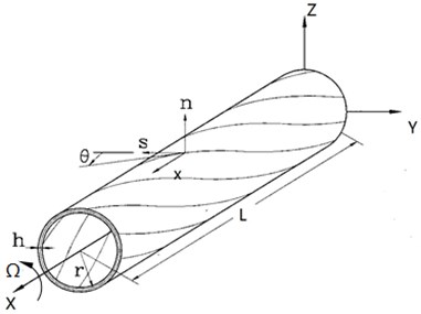
In the present study the composite shaft rotating along its longitudinal $x$ -axis at a constant rate $Ω$ is shown in Fig. 1. To describe the motion of the shaft the following coordinate systems are considered: (1) $(X, Y, Z)$ is inertial reference system whose origin $O$ is located in the geometric center, (2) $(x, y, z)$ is rotating reference system with the common origin $O .$ $(I, J, K)$ and $(i, j, k)$ denote the unit vectors of the reference systems $(X, Y, Z)$ and $(x, y, z),$ respectively. In addition a local coordinate system $(ξ, s, x)$ is used, where $ξ$ and $s$ are measured along the directions normal and tangent to the middle surface respectively.

The structural modeling is based on the following assumptions: (1) the shaft is characterized as a slender thin-walled elastic cylinder, satisfying $d ≪ L$ , $h ≪ d$ , $h ≪ r$ , where $L$ , $h$ , $r$ and $d$ denote the length, the thickness, the radius of curvature and the maximum cross sectional dimension of the cylinder respectively, (2) transverse shear effects are considered, (3) the loop stress resultant may be ignored, (4) a special laminated composite configuration, referred to as the circumferentially uniform stiffness configuration (CUS) achieved by skewing angle plies with respect to the longitudinal beam axis meeting the conditions $θ (y) = θ (- y)$ , $θ (z) = θ (- z)$ , is considered (Fig. 1).

Fig. 1Composite thin-walled shaft of a circular cross section

It has been shown [10-12] that VAM is an asymptotically correct theory which can be used effectively for the analysis of tubular composite thin-walled structures. However, the classical VAM does not account for the effects of transverse shear because of which it may generate inaccurate predictions of the rotating composite shaft. Herein the original formulation of VAM is expanded and refined to include effects of transverse shear of the composite shaft.

The displacement field incorporating shear deformation is assumed in the form:

1

u_{1} (x, y, z, t) = U_{1} (x, t) - y (s) θ_{y} (x, t) - z (s) θ_{z} (x, t) + g (s, x, t),

u_{2} (x, y, z, t) = U_{2} (x, t) - z ϕ (x, t),

u_{3} (x, y, z, t) = U_{3} (x, t) + y ϕ (x, t),

in which:

2

θ_{y} (x, t) = U_{2}^{'} (x, t) - 2 γ_{z x},

θ_{z} (x, t) = U_{3}^{'} (x, t) - 2 γ_{y x},

where $U_{1} (x, t), U_{2} (x, t), U_{3} (x, t)$ denote the rigid-body translations along the $x$ -, $y$ - and $z$ -axis, while $ϕ (x, t), θ_{y} (x, t), θ_{z} (x, t)$ denote the twist about the $z$ -axis and rotations about the $x$ - and $y$ -axis respectively. $γ_{z x}$ and $γ_{y x}$ denote the transverse shear strains in the planes $x z$ and $x y$ respectively.

From the classical VAM the warping function $g (s, x, t)$ is modified as:

3

g (s, x, t) = G (s) ϕ^{'} (x, t) + g_{1} (s) U_{1}^{'} (x, t) + g_{2} (s) θ_{y}^{'} (x, t) + g_{3} (s) θ_{z}^{'} (x, t) .

In the above equation the functions $g_{1} (s), g_{2} (s), g_{3} (s), G (s)$ are associated with physical behavior for the axial strain, the bending curvatures, and the torsion twist rate respectively. The primes in Eqs. (1) and (2) denote differentiation with respect to $x$ .

Based on the displacement representations (1), (2) and (3), and using the linear strain-displacement relations [9], while referring to the [13], the strain of the composite shaft can be written as:

4

γ_{x x} = U_{1}^{'} (x, t) - y θ_{y}^{'} (x, t) - z θ_{z}^{'} (x, t),

2 γ_{x s} = \frac{d g}{d s} + r_{n} ϕ^{'} + (U_{2}^{'} (x, t) - θ_{y} (x, t)) \frac{d y}{d s} + (U_{3}^{'} (x, t) - θ_{z} (x, t)) \frac{d z}{d s},

2 γ_{x ξ} = (U_{2}^{'} (x, t) - θ_{y} (x, t)) \frac{d z}{d s} - (U_{3}^{'} (x, t) - θ_{z} (x, t)) \frac{d y}{d s},

where $r_{n}$ denotes the project of the position vector $r$ of an arbitrary point on the cross-section of the deformed shaft in the normal direction:

5

r_{n} = y \frac{d z}{d s} - z \frac{d y}{d s} .

The position vector $r$ can be expressed as:

6

r = (y + u_{2}) i + (z + u_{3}) j + (x + u_{1}) k .

According to the constant rotating rate assumption and using the expressions for the time derivatives of unit vectors, one can obtain the velocity of a generic point as:

7

V = \dot{r} = ({\dot{u}}_{2} - Ω (z + u_{3})) i + ({\dot{u}}_{3} + Ω (y + u_{2})) j + {\dot{u}}_{1} k .

The strain energy of the composite shaft $U_{s}$ can be written as:

8

U_{s} = \frac{1}{2} \int_{0}^{L} \iint_{A}^{} (σ_{x x} ε_{x x} + σ_{x s} ε_{x s} + σ_{x ξ} ε_{x ξ}) d A d x,

where $σ_{x x},$ $σ_{x s}$ and $σ_{x ξ}$ represent the engineering stresses associated with the engineering strains $ε_{x x}$ , $ε_{x s}$ and $ε_{x ξ}$ .

Taking variation for the above strain energy expression one obtains:

9

δ U_{s} = \int_{0}^{L} \int_{A}^{} {(σ}_{x x} δ ε_{x x} + σ_{x s} δ ε_{x s} + σ_{x ξ} δ ε_{x ξ}) d A d x = \int_{0}^{L} [F_{x}^{'} δ U_{1} + Q_{y}^{'} δ U_{2} + Q_{z}^{'} δ U_{3} + M_{x}^{'} δ ϕ + (M_{z}^{'} + Q_{y}) δ θ_{y} + (M_{y}^{'} + Q_{z}) δ θ_{z}] d x .

Stress resultants $F_{x}$ , $Q_{y}$ , $Q_{z}$ and stress couples $M_{x}$ , $M_{y}$ , $M_{z}$ can be defined as:

10

F_{x} = \oint N_{x x} d s,

M_{x} = \oint N_{x s} r_{n} d s, M_{y} = - \oint N_{x x} z d s, M_{z} = - \oint N_{x x} y d s,

Q_{y} = \oint (N_{x s} \frac{d y}{d s} + N_{x ξ} \frac{d z}{d s}) d s, Q_{Z} = \oint (N_{x s} \frac{d z}{d s} - N_{x ξ} \frac{d y}{d s}) d s,

where $N_{x x}$ , $N_{x s}$ and $N_{x ξ}$ are shell stress resultants defined according to the following expressions:

11

[\begin{matrix} N_{x x} \\ N_{x s} \end{matrix}] = [\begin{matrix} A (s) & \frac{B (s)}{2} \\ \frac{B (s)}{2} & \frac{C (s)}{4} \end{matrix}] [\begin{matrix} γ_{x x} \\ {2 γ}_{x s} \end{matrix}],

N_{x ξ} = D (s) γ_{x ξ},

where:

12

A (s) = A_{11} - \frac{A_{12}^{2}}{A_{22}}, B (s) = 2 (A_{16} - \frac{A_{12} A_{26}}{A_{22}}),

C (s) = 4 [A_{66} - \frac{{{(A}_{26})}^{2}}{A_{22}}], D (s) = (A_{44} - \frac{A_{45}^{2}}{A_{55}}),

A_{i j} = \sum_{k = 1}^{N} {\bar{Q}}_{i j}^{(k)} (Z_{k} - Z_{k - 1}), (i, j = 1,2, 6; i, j = 4,5) .

Parameters $A (s)$ and $B (s)$ denote the reduced axial and coupling stiffnesses respectively, while $C (s)$ and $D (s)$ denote the reduced shear stiffnesses. $A_{i j}$ denote the in-plane stiffnesses components and ${\bar{Q}}_{i j}^{(k)}$ denote transformed stiffnesses.

Moreover by taking into account of Eqs. (4) and (11), the stress resultants and stress couples given by Eqs. (10) can be expressed in the following form:

13

F_{x} = k_{11} U_{1}^{'} + k_{12} ϕ^{'} + k_{13} θ_{z}^{'} + k_{14} θ_{y}^{'} + k_{15} (U_{2}^{'} - θ_{y}) + k_{16} (U_{3}^{'} - θ_{z}),

M_{x} = k_{12} U_{1}^{'} + k_{22} ϕ^{'} + k_{23} θ_{z}^{'} + k_{24} θ_{y}^{'} + k_{25} (U_{2}^{'} - θ_{y}) + k_{26} (U_{3}^{'} - θ_{z}),

M_{y} = k_{13} U_{1}^{'} + k_{23} ϕ^{'} + k_{33} θ_{z}^{'} + k_{34} θ_{y}^{'} + k_{35} (U_{2}^{'} - θ_{y}) + k_{36} (U_{3}^{'} - θ_{z}),

M_{z} = k_{14} U_{1}^{'} + k_{24} ϕ^{'} + k_{34} θ_{z}^{'} + k_{44} θ_{y}^{'} + k_{45} (U_{2}^{'} - θ_{y}) + k_{46} (U_{3}^{'} - θ_{z}),

Q_{y} = k_{51} U_{1}^{'} + k_{52} ϕ^{'} + k_{53} θ_{z}^{'} + k_{54} θ_{y}^{'} + k_{55} (U_{2}^{'} - θ_{y}) + k_{56} (U_{3}^{'} - θ_{z}),

Q_{z} = k_{61} U_{1}^{'} + k_{62} ϕ^{'} + k_{63} θ_{z}^{'} + k_{64} θ_{y}^{'} + k_{65} (U_{2}^{'} - θ_{y}) + k_{66} (U_{3}^{'} - θ_{z}),

where $k_{i j} (i, j = 1, \dots, 6)$ are the stiffness coefficients of the composite shaft, which can be expressed in terms of the cross sectional geometry and material properties as:

14

k_{11} = \oint_{Γ}^{} (A - \frac{B^{2}}{C}) d s + \{{[\oint_{Γ}^{} (\frac{B}{C}) d s]}^{2} / \oint_{Γ}^{} (\frac{1}{C}) d s\},

k_{12} = [\oint_{Γ}^{} (\frac{B}{C}) d s / \oint_{Γ}^{} (\frac{1}{C}) d s] A_{e},

k_{13} = - \oint_{Γ}^{} (A - \frac{B^{2}}{C}) z d s - \{[\oint_{Γ}^{} (\frac{B}{C}) d s \oint_{Γ}^{} (\frac{B}{C}) z d s] / \oint_{Γ}^{} (\frac{1}{C}) d s\},

k_{14} = - \oint_{Γ}^{} (A - \frac{B^{2}}{C}) y d s - \{[\oint_{Γ}^{} (\frac{B}{C}) d s \oint_{Γ}^{} (\frac{B}{C}) y d s] / \oint_{Γ}^{} (\frac{1}{C}) d s\},

k_{22} = [1 / \oint_{Γ}^{} (\frac{1}{C}) d s] A_{e}^{2},

k_{23} = - [\oint_{Γ}^{} (\frac{B}{C}) z d s / \oint_{Γ}^{} (\frac{1}{C}) d s] A_{e},

k_{24} = - [\oint_{Γ}^{} (\frac{B}{C}) y d s / \oint_{Γ}^{} (\frac{1}{C}) d s] A_{e},

k_{33} = \oint_{Γ}^{} (A - \frac{B^{2}}{C}) z^{2} d s + \{{[\oint_{Γ}^{} (\frac{B}{C}) z d s]}^{2} / \oint_{Γ}^{} (\frac{1}{C}) d s\},

k_{34} = \oint_{Γ}^{} (A - \frac{B^{2}}{C}) y z d s + \{[\oint_{Γ}^{} (\frac{B}{C}) y d s \oint_{Γ}^{} (\frac{B}{C}) z d s] / \oint_{Γ}^{} (\frac{1}{C}) d s\},

k_{44} = \oint_{Γ}^{} (A - \frac{B^{2}}{C}) y^{2} d s + \{{[\oint_{Γ}^{} (\frac{B}{C}) y d s]}^{2} / \oint_{Γ}^{} (\frac{1}{C}) d s\},

k_{15} = \frac{1}{2} \oint_{Γ}^{} B \frac{d y}{d s} d s, k_{16} = \frac{1}{2} \oint_{Γ}^{} B \frac{d z}{d s} d s, k_{25} = \frac{1}{4} \oint_{Γ}^{} r_{n} C \frac{d y}{d s} d s,

k_{26} = \frac{1}{4} \oint_{Γ}^{} r_{n} C \frac{d z}{d s} d s, k_{35} = - \frac{1}{2} \oint_{Γ}^{} B z \frac{d y}{d s} d s, k_{36} = - \frac{1}{2} \oint_{Γ}^{} B z \frac{d z}{d s} d s,

k_{45} = - \frac{1}{2} \oint_{Γ}^{} B y \frac{d y}{d s} d s, k_{46} = - \frac{1}{2} \oint_{Γ}^{} B y \frac{d z}{d s} d s,

k_{55} = \oint_{Γ}^{} [\frac{1}{4} {C (\frac{d y}{d s})}^{2} + {D (\frac{d z}{d s})}^{2}] d s, k_{56} = \oint_{Γ}^{} (\frac{1}{4} C - D) \frac{d y}{d s} \frac{d z}{d s} d s,

k_{66} = \oint_{Γ}^{} [\frac{1}{4} {C (\frac{d z}{d s})}^{2} + {D (\frac{d y}{d s})}^{2}] d s .

The coefficients $k_{i j} (i, j = 1,2, \dots, 4)$ represent the stiffnesses, as described in [9, 12] for the case of a non-shearable thin-walled beam, while the shear contribution to the stiffness coefficients is represented by the new terms $k_{i j} (i = 1,2, \dots, 6; j = 5,6)$ , $k_{j i} (i = 1,2, \dots, 4; j = 5,6)$ .

The kinetic energy of the composite shaft $T_{s}$ can be written as:

15

T_{s} = \frac{1}{2} \int_{0}^{L} \iint_{A}^{} ρ (V \cdot V) d A d x,

where $ρ$ denotes the mass density of the shaft. In view of Eq. (7) the expression of the kinetic energy can be obtained and taking variation of $T_{s}$ yields:

16

δ T_{s} = - \int_{0}^{L} (I_{1} δ U_{1} + I_{2} δ U_{2} {+ I}_{3} δ U_{3} + I_{4} δ θ_{y} + I_{5} δ θ_{z} {+ I}_{6} δ ϕ),

where:

17

I_{1} = b_{1} {\ddot{U}}_{1} - b_{2} {\ddot{θ}}_{y} - b_{3} {\ddot{θ}}_{x},

I_{2} = b_{1} ({\ddot{U}}_{2} - 2 Ω {\dot{U}}_{3} - Ω^{2} U_{2}) - b_{2} (2 Ω \dot{ϕ} + Ω^{2}) - b_{3} (\ddot{ϕ} - Ω^{2} ϕ),

I_{3} = b_{1} ({\ddot{U}}_{3} + 2 Ω {\dot{U}}_{2} - Ω^{2} U_{3}) + b_{2} (\ddot{ϕ} - Ω^{2} ϕ) - b_{3} (2 Ω \dot{ϕ} + Ω^{2}),

I_{4} = b_{2} {\ddot{U}}_{1} - b_{4} {\ddot{θ}}_{y} - b_{6} {\ddot{θ}}_{z},

I_{5} = b_{3} {\ddot{U}}_{3} - b_{6} {\ddot{θ}}_{y} - b_{5} {\ddot{θ}}_{z},

I_{6} = b_{2} ({\ddot{U}}_{3} + 2 Ω {\dot{U}}_{2} - Ω^{2} U_{3}) + (b_{4} + b_{5}) (\ddot{ϕ} - Ω^{2} ϕ) - b_{3} ({\ddot{U}}_{2} - 2 Ω {\dot{U}}_{3} - Ω^{2} U_{2}),

b_{1} = \iint_{A}^{} ρ d A, b_{2} = \iint_{A}^{} ρ y d A, b_{3} = \iint_{A}^{} ρ z d A,

b_{4} = \iint_{A}^{} ρ y^{2} d A, b_{5} = \iint_{A}^{} ρ z^{2} d A, b_{6} = \iint_{A}^{} ρ y z d A .

2.2. Kinetic energy of rigid disks

According to Eqs. (16) and (17) the expression of variation of the kinetic energy of the rigid disks fixed to the shaft is written as:

18

δ T_{D} = - \int_{0}^{L} (\sum_{l = 1}^{N_{D}} (I_{1 l}^{D} δ U_{1} + I_{2 l}^{D} δ U_{2} + I_{3 l}^{D} δ U_{3} + I_{4 l}^{D} δ θ_{y} + I_{5 l}^{D} δ θ_{z} + I_{6 l}^{D} δ ϕ) Δ (x - x_{D l})) d x,

in which:

19

I_{1 l}^{D} = b_{1 l}^{D} {\ddot{U}}_{1} - b_{2 l}^{D} {\ddot{θ}}_{y} - b_{3 l}^{D} {\ddot{θ}}_{Z},

I_{2 l}^{D} = b_{1 l}^{D} ({\ddot{U}}_{2} - 2 Ω {\dot{U}}_{3} - Ω^{2} U_{2}) - b_{2 l}^{D} (2 Ω \dot{ϕ} + Ω^{2}) - b_{3 l}^{D} (\ddot{ϕ} - Ω^{2} ϕ),

I_{3 l}^{D} = b_{1 l}^{D} ({\ddot{U}}_{3} + 2 Ω {\dot{U}}_{2} - Ω^{2} U_{3}) + b_{2 l}^{D} (\ddot{ϕ} - Ω^{2} ϕ) - b_{3 l}^{D} (2 Ω \dot{ϕ} + Ω^{2}),

I_{4 l}^{D} = b_{2 l}^{D} {\ddot{U}}_{1} - b_{4 l}^{D} {\ddot{θ}}_{y} - b_{6 l}^{D} {\ddot{θ}}_{Z},

I_{5 l}^{D} = b_{3 l}^{D} {\ddot{U}}_{3} - b_{6 l}^{D} {\ddot{θ}}_{y} - b_{5 l}^{D} {\ddot{θ}}_{Z},

I_{6 l}^{D} = b_{2 l}^{D} ({\ddot{U}}_{3} + 2 Ω {\dot{U}}_{2} - Ω^{2} U_{3}) + (b_{4 l}^{D} + b_{5 l}^{D}) (\ddot{ϕ} - Ω^{2} ϕ) - b_{3 l}^{D} ({\ddot{U}}_{2} - 2 Ω {\dot{U}}_{3} - Ω^{2} U_{2}),

b_{1 l}^{D} = \iint_{A}^{} ρ_{l}^{D} d A, b_{2 l}^{D} = \iint_{A}^{} ρ_{l}^{D} y d A, b_{3 l}^{D} = \iint_{A}^{} ρ_{l}^{D} z d A,

b_{4 l}^{D} = \iint_{A}^{} ρ_{l}^{D} y^{2} d A, b_{5 l}^{D} = \iint_{A}^{} ρ_{l}^{D} z^{2} d A, b_{6 l}^{D} = \iint_{A}^{} ρ_{l}^{D} y z d A,

where $ρ_{l}^{D}$ denotes the mass density of the disk $l$ . The symbol $Δ (x - x_{D l})$ denotes Dirac delta function, $N_{D}$ the number of the disks mounted on the shaft and $x_{D l}$ the location of the $l$ th disk.

2.3. Work of external forces

The external forces include the centrifugal force resulting from the unbalanced rigid disks and the force from the bearings.

The bearings are considered as the springs and viscous dampers and these elements have linear stiffness and damping characteristics.

The virtual work associated with the springs and viscous dampers can be expressed as:

20

{δ W}_{b} = \int_{0}^{L} [\sum_{l = 1}^{n_{b}} (\begin{matrix} - K_{y y}^{b l} U_{2} δ U_{2} - K_{z y}^{b l} U_{2} δ U_{3} - K_{y z}^{b l} U_{3} δ U_{2} - K_{z z}^{b l} U_{3} δ U_{3} \\ - C_{y y}^{b l} {\dot{U}}_{2} δ {\dot{U}}_{2} - C_{z y}^{b l} {\dot{U}}_{2} δ {\dot{U}}_{3} {- C}_{y z}^{b l} {\dot{U}}_{3} δ {\dot{U}}_{2} - C_{z z}^{b l} {\dot{U}}_{3} δ {\dot{U}}_{3} \end{matrix}) Δ (x - x_{b l})] d x,

where $n_{b}$ denotes the number of the bearings, $x_{b l}$ the location, $K^{b l}$ and $C^{b l}$ the equivalent stiffness and damping coefficients of the $l$ th bearings.

The virtual work done by the centrifugal force of rigid disks can be given by:

$δ W_{e} = \int_{0}^{L} (p_{x}^{u} δ U_{1} + p_{y}^{u} δ U_{2} + p_{z}^{u} δ U_{3} + Γ_{x}^{u} δ ϕ + Γ_{y}^{u} δ θ_{y} + Γ_{z}^{u} δ θ_{z}) d x,$

where $p_{x}^{u}$ , $p_{y}^{u}$ , $p_{z}^{u}$ denote centrifugal force per unit length, $Γ_{x}^{u}$ , $Γ_{y}^{u}$ , $Γ_{z}^{u}$ denote centrifugal moment per unit length. They are given by:

21

p_{x}^{u} = 0, p_{y}^{u} = Ω^{2} (c o s Ω t) \sum_{l = 1}^{N_{D}} b_{1 l}^{D} e_{l} Δ (x - x_{D l}), p_{z}^{u} = Ω^{2} (s i n Ω t) \sum_{l = 1}^{N_{D}} b_{1 l}^{D} e_{l} Δ (x - x_{D l}),

Γ_{x}^{u} = 0, Γ_{y}^{u} = 0, Γ_{z}^{u} = 0,

where the mass unbalance associated with disks is assumed as the concentrated masses $b_{1 l}^{D} = \iint_{A}^{} ρ_{l}^{D} d A$ at points with small distances of eccentricity $e_{l}$ .

2.4. Motion equations of systems

In view of Eqs. (9), (16), (28) and (30), and employing the following variational principle:

22

\int_{t_{0}}^{t_{1}} [δ U_{s} - δ (T_{s} + T_{D}) - δ W_{b} - δ W_{e}] d t = 0,

one obtains:

23

- F_{x}^{'} + I_{1} + I_{1}^{D} = p_{x}^{u},

- Q_{y}^{'} + I_{2} + I_{2}^{D} + F_{U_{2}}^{b} = p_{y}^{u},

- Q_{z}^{'} + I_{3} + I_{3}^{D} + F_{U_{3}}^{b} = p_{z}^{u},

- M_{x}^{'} + I_{6} + I_{6}^{D} = Γ_{x}^{u},

- M_{z}^{'} + I_{4} + I_{4}^{D} = Γ_{y}^{u},

- M_{y}^{'} + I_{5} + I_{5}^{D} = Γ_{z}^{u},

where:

24

F_{U_{2}}^{b} = \sum_{l = 1}^{n_{b}} (K_{y y}^{b l} U_{2} + K_{y z}^{b l} U_{3} + K_{y y}^{b l} {\dot{U}}_{2} + K_{y z}^{b l} {\dot{U}}_{3}) Δ (x - x_{b l}),

F_{U_{3}}^{b} = \sum_{l = 1}^{n_{b}} (K_{z z}^{b l} U_{3} + K_{z y}^{b l} U_{2} + K_{z z}^{b l} {\dot{U}}_{3} + K_{z y}^{b l} {\dot{U}}_{2}) Δ (x - x_{b l}) .

The boundary conditions at $x = 0$ , $L$ are:

25

F_{x} = {\bar{F}}_{x} o r U_{1} = {\bar{U}}_{1}, Q_{y} = {\bar{Q}}_{y} o r U_{2} = {\bar{U}}_{2}, Q_{z} = {\bar{Q}}_{z} o r U_{3} = {\bar{U}}_{3},

M_{x} = {\bar{M}}_{x} o r θ_{y} = {\bar{θ}}_{y}, M_{y} = {\bar{M}}_{y} o r θ_{z} = {\bar{θ}}_{z}, M_{z} = {\bar{M}}_{z} o r ϕ = \bar{ϕ} .

As a result of CUS configuration, the equations of motion involving variables in terms of displacements can be reduced and split into two independent equation systems associated with both bending-transverse shear and extension-twist motions.

The motion equations of bending-transverse shear coupling:

26

- k_{35} θ_{z}^{''} - k_{55} (U_{2}^{''} - θ_{y}^{'}) + b_{1} ({\ddot{U}}_{2} - 2 Ω {\dot{U}}_{3} - Ω^{2} U_{2})

+ \sum_{l = 1}^{N_{D}} [b_{1 l}^{D} ({\ddot{U}}_{2} - 2 Ω {\dot{U}}_{3} - Ω^{2} U_{2})] (x - x_{D l}) + F_{U_{2}}^{b} = p_{y}^{u},

- k_{46} θ_{y}^{''} - k_{66} (U_{3}^{''} - θ_{z}^{'}) + b_{1} ({\ddot{U}}_{3} + 2 Ω {\dot{U}}_{2} - Ω^{2} U_{3}) + \sum_{l = 1}^{N_{D}} [b_{1 l}^{D} ({\ddot{U}}_{3} + 2 Ω {\dot{U}}_{2} - Ω^{2} U_{3})] (x - x_{D l}) + F_{U_{3}}^{b} = p_{z}^{u},

- k_{44} θ_{y}^{''} - k_{46} (U_{3}^{''} - θ_{z}^{'}) - k_{35} θ_{z}^{'} - k_{55} (U_{2}^{'} - θ_{y}^{}) - b_{4} {\ddot{θ}}_{y} + \sum_{l = 1}^{N_{D}} ({- b}_{4 l}^{D} {\ddot{θ}}_{y}^{}) Δ (x - x_{D l}) = 0,

- k_{33} θ_{z}^{''} - k_{35} (U_{2}^{''} - θ_{y}^{'}) - k_{46} θ_{y}^{'} - k_{66} (U_{3}^{'} - θ_{z}^{}) - b_{5} {\ddot{θ}}_{z} + \sum_{l = 1}^{N_{D}} ({- b}_{5 l}^{D} {\ddot{θ}}_{z}^{}) Δ (x - x_{D l}) = 0 .

The motion equations of extension-twist coupling:

27

- k_{11} U_{1}^{''} - k_{12}^{} ϕ^{''} + b_{1} {\ddot{U}}_{1} = 0,

- k_{12} U_{1}^{''} - k_{22} ϕ^{''} + (b_{4} + b_{5}) (\ddot{ϕ} - Ω^{2} ϕ) = 0 .

By using the coordinate transformation Eq. (26) can be transformed to the inertia reference frame $(X, Y, Z)$ . The results are not presented in this paper for the sake of simplicity.

In present study emphasis is placed on only the problem involving the bending-transverse shear coupling.

2.5. Approximate solution method

In order to find the approximate solution of the rotating composite shaft, the quantities $U_{2} (x, t)$ , $U_{3} (x, t)$ , $θ_{y} (x, t)$ and $θ_{z} (x, t)$ are assumed in the form:

28

U_{2} (x, t) = \sum_{j = 1}^{N} U_{j} (t) α_{j} (x), U_{3} (x, t) = \sum_{j = 1}^{N} U_{j} (t) α_{j} (x),

θ_{y} (x, t) = \sum_{j = 1}^{N} Θ_{j} (t) ψ_{j} (x), θ_{z} (x, t) = \sum_{j = 1}^{N} Θ_{j} (t) ψ_{j} (x),

where $α_{j} (x)$ and $ψ_{j} (x)$ denote mode shape functions which fulfill all the boundary conditions of the composite shaft, $U_{j} (t)$ and $Θ_{j} (t)$ are the generalized coordinates.

Substituting Eq. (28) into the governing Eq. (26) and applying Galerkin’s procedure, the following governing equations in matrix form can be found:

29

[M] \{\ddot{X}\} + [C] \{\dot{X}\} + ([K_{Ω}] + [K_{1}]) \{X\} = \{f\},

where $[M]$ denotes the mass matrix, $[C]$ the gyroscopic matrix, $[K_{1}]$ the elastic stiffness matrix, $[K_{Ω}]$ stiffness matrix which depends on the rotational speed $Ω$ , $\{f\}$ the generalized force vector. $\{\ddot{X}\},$ $\{\dot{X}\}$ and $\{X\}$ denote the generalized acceleration, velocity and displacement vectors respectively.

These matrices can be written as follows:

30

[M] = [\begin{matrix} b_{1} E_{i j} + \sum_{l = 1}^{N_{D}} b_{1 l}^{D} E_{i j}^{D l} & 0 & 0 & 0 \\ 0 & b_{1} E_{i j} + \sum_{l = 1}^{N_{D}} b_{1 l}^{D} E_{i j}^{D l} & 0 & 0 \\ 0 & 0 & - b_{4} F_{i j} - \sum_{l = 1}^{N_{D}} b_{4 l}^{D} F_{i j}^{l} & 0 \\ 0 & 0 & 0 & - b_{5} F_{i j} - \sum_{l = 1}^{N_{D}} b_{5 l}^{D} F_{i j}^{l} \end{matrix}],

31

[C] = [\begin{matrix} \sum_{l = 1}^{N_{D}} C_{y y}^{b l} E_{i j}^{b l} & (\begin{matrix} - 2 Ω b_{1} E_{i j} - 2 Ω \sum_{l = 1}^{N_{D}} b_{1 l}^{D} E_{i j}^{D l} \\ + \sum_{l = 1}^{N_{D}} C_{y z}^{b l} E_{i j}^{b l} \end{matrix}) & 0 & 0 \\ 2 Ω b_{1} E_{i j} - 2 Ω \sum_{l = 1}^{N_{D}} b_{1 l}^{D} E_{i j}^{D l} + \sum_{l = 1}^{N_{D}} C_{z y}^{b l} E_{i j}^{b l} & \sum_{l = 1}^{N_{D}} C_{z z}^{b l} E_{i j}^{b l} & 0 & 0 \\ 0 & 0 & 0 & 0 \\ 0 & 0 & 0 & 0 \end{matrix}],

32

[K_{Ω}] = [\begin{matrix} - b_{1} Ω^{2} E_{i j} - Ω^{2} \sum_{l = 1}^{N_{D}} b_{1 l}^{D} E_{i j}^{D l} & 0 & 0 & 0 \\ 0 & - b_{1} Ω^{2} E_{i j} - Ω^{2} \sum_{l = 1}^{N_{D}} b_{1 l}^{D} E_{i j}^{D l} & 0 & 0 \\ 0 & 0 & 0 & 0 \\ 0 & 0 & 0 & 0 \end{matrix}],

33

[K_{1}] = [\begin{matrix} - k_{55} I_{i j} + \sum_{l = 1}^{N_{D}} {K_{y y}^{b l}}_{} E_{i j}^{b l} & \sum_{l = 1}^{N_{D}} {K_{y z}^{b l}}_{} E_{i j}^{b l} & k_{55} J_{i j} & - k_{35} K_{i j} \\ \sum_{l = 1}^{N_{D}} {K_{z y}^{b l}}_{} E_{i j}^{b l} & - k_{66} I_{i j} + \sum_{l = 1}^{N_{D}} {K_{z z}^{b l}}_{} E_{i j}^{b l} & - k_{46} K_{i j} & k_{66} J_{i j} \\ - k_{55} O_{i j} & - k_{46} P_{i j} & - k_{44} Q_{i j} + k_{55} F_{i j} & 0 \\ {- k}_{35} P_{i j} & {- k}_{66} O_{i j} & 0 & - k_{33} Q_{i j} + k_{66} F_{i j} \end{matrix}],

34

{\{f\}}^{T} = Ω^{2} \sum_{l = 1}^{N_{D}} b_{1 l}^{D} e_{l} B_{i}^{D l} {(\cos Ω t \sin Ω t 0 0)}_{1 \times 4 N},

where:

35

E_{i j} = \int_{0}^{L} α_{i} α_{j} d x, F_{i j} = \int_{0}^{L} ψ_{i} ψ_{j} d x, E_{i j}^{D l} = \int_{0}^{L} α_{i} α_{j} Δ (x - x_{D l}) d x,

F_{i j}^{D l} = \int_{0}^{L} ψ_{i} ψ_{j} Δ (x - x_{D l}) d x, E_{i j}^{b l} = \int_{0}^{L} α_{i} α_{j} Δ (x - x_{b l}) d x, I_{i j} = \int_{0}^{L} α_{i} α_{j}^{''} d x,

J_{i j} = \int_{0}^{L} α_{i} ψ_{j}^{'} d x, K_{i j}^{} = \int_{0}^{L} α_{i} ψ_{j}^{''} d x, O_{i j} = \int_{0}^{L} ψ_{i} α_{j}^{'} d x, P_{i j} = \int_{0}^{L} ψ_{i} α_{j}^{''} d x,

Q_{i j} = \int_{0}^{L} ψ_{i} ψ_{j}^{''} d x, B_{i}^{D l} = \int_{0}^{L} α_{i} Δ (x - x_{D l}) d x, (i, j = 1,2, \dots, N) .

The above approximate equations of the motion (29) can be easily simplified as the generalized eigenvalue problem. So the free vibration, stability and response of the composite shaft system can be studied by the eigenvalue equation. The resulting equation is not presented for the sake of simplicity.

3. Numerical simulations

3.1. Model verifications

In order to examine the influence of the number of mode shape functions used in the solution of the equation on the accuracy of the results, the numerical results of natural frequencies are shown in Table 1 for an increasing number of mode shape functions. From Table 1 it can be seen that to obtain accurate results of the first three natural frequencies, no more than six mode shape functions are required. This indicates clearly that the convergence of the present model is quite good.

The natural frequencies of a cantilever composite shaft obtained for the problem without shear deformation using the present model together with those obtained in [14] are shown in Table 2 for different rotating speeds. A perfect agreement of numerical results with those in [14] can be seen.

Table 1Effect of model number N on natural frequencies (Ω*= 0 and θ= 30°)

$N$	$ω_{1}^{*}$	$ω_{2}^{*}$	$ω_{3}^{*}$	$ω_{4}^{*}$	$ω_{5}^{*}$	$ω_{6}^{*}$
2	2.99	11.87	-	-	-	-
4	2.98	11.68	25.17	42.41	-	-
6	2.97	11.65	25.12	41.90	60.29	80.02
8	2.97	11.64	25.10	41.84	60.21	79.22
10	2.97	11.64	25.09	41.82	60.18	79.14

Table 2Comparison of the natural frequencies of a cantilever composite shaft without shear deformation

$Ω^{*}$	$ω_{1}^{*}$	$ω_{2}^{*}$	$ω_{3}^{*}$	$ω_{4}^{*}$	$ω_{5}^{*}$	$ω_{6}^{*}$
0	3.5160	3.5160	22.0345	22.0345	61.6973	61.6973
Ref. [14]	3.5160	3.5160	22.0340	22.0340	61.6970	61.6970
2	1.5160	5.5160	20.0345	24.0345	59.6973	69.6973
Ref. [14]	1.5160	5.5160	20.0340	24.0340	59.6970	63.6970
3.5	0.0160	7.0160	18.5345	25.5345	58.1973	65.1973
Ref. [14]	0.0000	7.0160	18.5340	25.5340	58.1970	65.1970
4	-	7.5160	18.0345	26.0345	57.6973	65.6973
Ref. [14]	-	7.5160	18.0340	26.0340	57.6970	65.6970
8	-	11.5160	14.0345	3.30345	53.6973	69.6973
Ref. [14]	-	11.5160	14.0340	30.0340	53.6970	69.6970

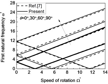
The variation of natural frequencies vs. rotating speed for simply supported shear shaft is shown in Fig. 2 from the present model with the ones from [7]. The numerical results are given in terms of the normalized natural frequencies and rotating rate that are defined by $ω^{*} = ω / ω_{0}$ , $Ω^{*} = Ω / ω_{0}$ , where the normalizing factor $ω_{0} =$ 138.85 rad/s is the fundamental frequency of the non-rotating shaft with $θ = 0 °$ .

From this figure it clearly appears that when $Ω^{*} =$ 0 a single zero-speed mode natural frequency is obtained. As the rotating speed $Ω^{*}$ is increased, due to the gyroscopic effect the natural frequencies ‘split’ into the upper and lower frequency branches. The upper frequency branch is associated with the forward whirling frequency (FW or F) motion. Similarly lower frequency branch is associated with the backward whirling frequency (BW or B) motion. The minimum rotating rate at which the BW frequency becomes zero is referred to as the critical rotating speed, which will cause the dynamically unstable motion of the rotating shaft. In addition to this, it can obviously be seen that the present numerical results are in good agreement with the results presented in [7].

Fig. 2The natural frequency of a simply supported composite shaft versus rotating speed for different ply angles

3.2. Results and discussion

In the following application the natural frequencies, critical rotating speeds and the unbalance response of a composite shaft system are computed using presented model. The composite rotor system is a composite shaft with one rigid disk supported by two bearings at the ends, the disk is at the mid-point of the shaft as shown in Fig. 3. The shaft geometrical properties are: $L =$ 2.47 m, $r =$ 0.0635 m, $h =$ 0.001321 m [15]. Ratio of length over radius of the shaft is 38.89764 and radius over thickness 48.10606, which are suitable for features of the slender thin-walled shaft and consistent with assumption as used in the present model. The shaft is made by boron-epoxy composite material with parameters as follows: $E_{11} = 2.11 GPa,$ $E_{22} = 24.1 GPa,$ $G_{12} = G_{13} = G_{23} =$ 6.9 GPa, $ν_{12} =$ 0.36, $ρ =$ 1967.0 kg/m³ [3]. The stacking sequence of the composite shaft is ${[\pm θ]}_{5}$ . The properties of the disk and the two bearings are given in Table 3.

Table 3The properties of disk and bearings [5]

	Disk	Bearings
$b_{1 l}^{D}$ (kg)	2.4364	-
$e$ (10^-5 m)	5.0000	-
$b_{4 l}^{D}, b_{5 l}^{D}$ (kg m²)	0.1901	-
$K_{y y}, K_{z z}$ (10⁷ N/m)	-	1.75
$C_{y y}, C_{z z}$ (10⁷ Ns/m)	-	5.00

Fig. 3The composite shaft system with bearings and disk

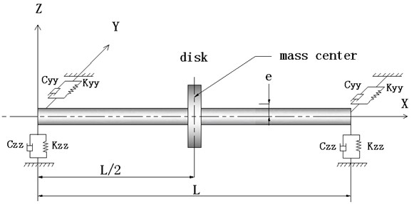
Fig. 4The Campbell diagram of a composite shaft system (θ= 0°)

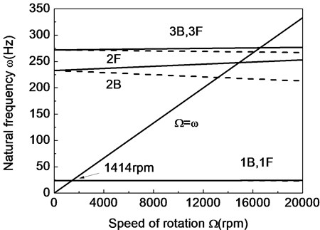
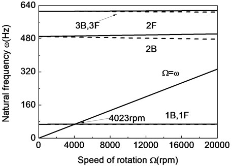
Fig. 5The Campbell diagram of a composite shaft system (θ= 60°)

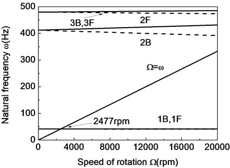
Fig. 6The Campbell diagram of a composite shaft system (θ= 90°)

Based on mode convergence examination it is found that $N =$ 5 gives suitably converged eigenvalues. So for all results given in this paper $N =$ 5 unless otherwise noted.

Figs. 4-6 present the Campbell diagrams which display the variation of the first three frequencies with respect to rotating speed for various fiber ply-angles. The crossover point of the straight line with BW curves yields the critical rotating speed of the composite shaft system. The predicted critical rotating speeds for the fiber ply-angles $θ =$ 0°, 60°, 90° are $Ω_{c r} =$ 1414 rpm, 2477 rpm and 4023 rpm respectively. The results show that non-rotating natural frequencies and the critical rotating speeds increase as fiber ply-angle increases. The reason is that the bending siffnesses $k_{33}$ and $k_{44}$ increase when fiber ply-angle increases.

Fig. 7The Campbell diagram of a composite shaft system (— with shear deformation; - - - without shear deformation)

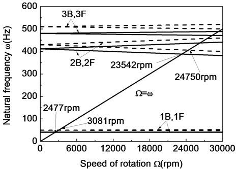
Fig. 8The first two critical speeds of a composite shaft system versus ratio of length over radius

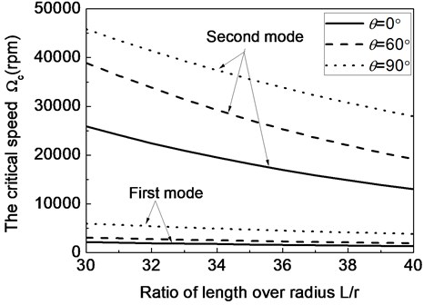
Fig. 9The first two critical speeds of a composite shaft system versus ratio of radius over thickness

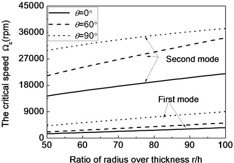
Fig. 7 presents the Campbell diagrams both with and without transversal shear effects. The critical rotating speeds predicted by the model with and without transversal shear deformation are found to be $Ω_{c r} =$ 2477 rpm and 3081 rpm for the first critical rotating speed and $Ω_{c r} =$ 23542 rpm and 24750 rpm for the second critical rotating speed respectively. The error of 24.38 % in the first critical rotating speed and 5.13 % in the second critical rotating speed can be observed for problems with and without shear effects. As a result, the classical composite thin-walled beams over-estimate the stability of composite shaft system.

Figs. 8 and 9 present the variation of critical rotating speed with respect to the shaft parameters $L / r$ (ratio of length over radius) and $r / h$ (ratio of radius over thickness) for different fiber ply-angles respectively. The results show that critical speeds decrease as $L / r$ increases, whereas they increase as $r / h$ increases.

Fig. 10The first two natural frequencies of a composite shaft system versus ratio of length over radius (Ω= 20000 rpm)

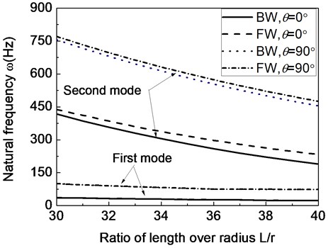
Fig. 11The first two natural frequencies of a composite shaft system versus ratio of radius over thickness (Ω= 20000 rpm)

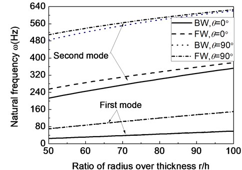
Figs. 10 and 11 present the variation of the first two natural frequencies with respect to the shaft parameters $L / r$ and $r / h$ for different fiber ply-angles respectively. Because of the influences of rotating speed ( $Ω =$ 20000 rpm) there are the upper and lower frequency branches for each whirling mode as shown in these figures.

From Figs. 10 and 11 it can be seen that the variations of natural frequencies with the parameters $L / r$ and $r / h$ are similar to that previously presented for the critical rotating speed. However, from these figures it is evident that rotating speed has much more influence on the higher-mode ones than the lower-mode ones.

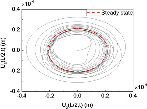
Fig. 12Trajectory of a composite shaft system for a transient unbalance load: a) undercritical rotating speed Ω= 3000 rpm; b) critical rotating speed Ω=Ωcr= 4023 rpm; c) supercritical rotating speed Ω= 5000 rpm

Trajectory of a composite shaft system for a transient unbalance load: a) undercritical rotating speed Ω= 3000 rpm; b) critical rotating speed Ω=Ωcr= 4023 rpm; c) supercritical rotating speed Ω= 5000 rpm

a)

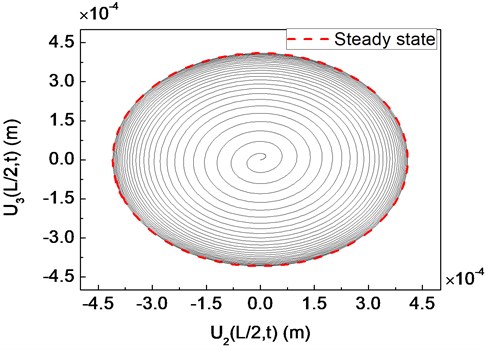
b)

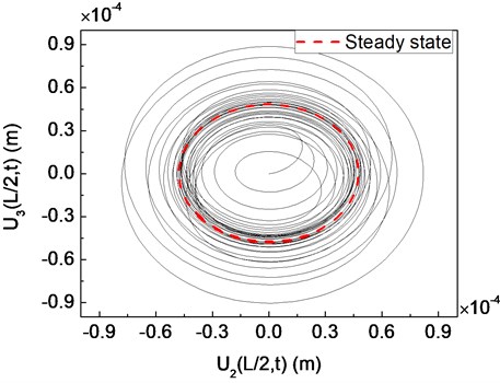
c)

Fig. 12 presents the trajectories of the geometric center of the rigid disk for various rotating speeds (3000, 4023 and 5000 rpm). It clearly shows that when rotating speed is equal to the critical rotating speed $Ω = Ω_{c r} =$ 4023 rpm, a violent whirling response occurs due to resonant vibration. It can also be noted that the forward mode of a supercritical composite shaft system is stable since the internal damping of the composite shaft is not taken into account in the presented model.

Fig. 13The time response of the displacement at the disk center: (a) U2(L/2,t); (b) U3(L/2,t)

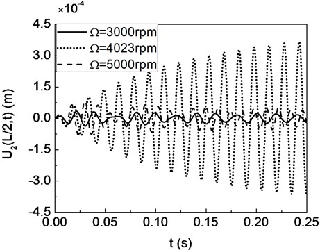
a)

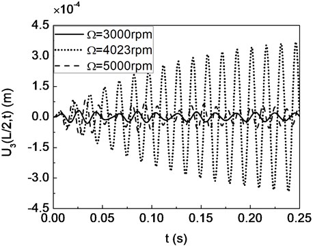
b)

Fig. 13 presents the time response of the displacement at the disk center which corresponds to that previously presented in Fig. 12. It can be seen from Fig. 12 and 13 that the unbalance responses arrive rapidly to the steady state vibration due to the external damping from bearings.

4. Conclusions

This paper deals with the structural modeling and dynamical analysis of rotating composite shaft. An analytical model capable of predicting of the natural frequency, the critical rotating speed and the unbalanced response of composite shaft system has been proposed based on the thin-walled composite beam theory referred to as VAM. Numerical simulations of the effects of various parameters including fiber ply-angle, geometric dimension and the transverse shear deformation on frequencies and critical rotating speeds are performed. The comparative study and the convergence examination of the approximate solution methodology show that the analytical model and numerical method developed in this paper can be used to highlight the dynamical behaviors of rotating composite shaft system. The present model can further be extended to incorporate the effects of internal damping of composite shaft for evaluating the dynamical instabilities due to internal damping. This improvement will be reported in the forthcoming paper.

References

Zinberg H., Symonds M. F. The development of an advanced composite tail rotor drive shaft. Presented at the 26th Annual National Forum of the American Helicopter Society, Washington, DC, 1970.

Search CrossRef
Dos Reis H. L. M., Goldman R. B., Verstrate P. H. Thin-walled laminated composite cylindrical tubes; Part III – Critical speed analysis. J. Compos. Technol. Res., Vol. 9, 1987, p. 58-62.

Search CrossRef
Kim C. D., Bert C. W. Critical speed analysis of laminated composite, hollow drive shafts. Composites Engineering, Vol. 3, 1993, p. 633-643.

Search CrossRef
Singh S. P., Gupta K. Composite shaft rotordynamic analysis using a layerwise theory. Journal of Sound and Vibration, Vol. 191, Issue 5, 1996, p. 739-756.

Search CrossRef
Chang M. Y., Chen J. K., Chang C. Y. A simple spinning laminated composite shaft model. International Journal of Solids and Structures, Vol. 41, 2004, p. 637-662.

Search CrossRef
Gubran H. B. H., Gupta K. The effect of stacking sequence and coupling mechanisms on the natural frequencies of composite shafts. Journal of Sound and Vibration, Vol. 282, 2005, p. 231-248.

Search CrossRef
Song O., Jeong N.-H., Librescu L. Implication of conservative and gyroscopic forces on vibration and stability of an elastically tailored rotating shaft modeled as a composite thin-walled beam. Journal of Acoustical Society of America, Vol. 109, Issue 3, 2001, p. 972-981.

Search CrossRef
Rehfield L. W. Design analysis methodology for composite rotor blades. Proc. Seventh DoD/NASA Conf. on Fibrous Composites in Structural Design, AFWAL-TR-85-3094, 1985.

Search CrossRef
Berdichevsky V. L., Armanios E., Badir A. M. Theory of anisotropic thin-walled closed-cross-section beams. Composites Engineering, Vol. 2, Issue 5-7, 1992, p. 411-432.

Search CrossRef
Park J. S., Kim J. H. Design and aeroelastic analysis of active twist rotor blades incorporating single crystal macro fiber composite actuators. Composites: Part B, Vol. 39, 2008, p. 1011-1025.

Search CrossRef
Cesnik C. E. S., Shin S. J. On the modeling of integrally actuated helicopter blades. International Journal of Solids and Structures, Vol. 38, 2001, p. 1765-1789.

Search CrossRef
Armanios E. A., Badir A. M. Free vibration analysis of anisotropic thin-walled closed-section beams. AIAA J., Vol. 33, Issue 10, 1995, p. 1905-1910.

Search CrossRef
Song O., Librescu L. Structural modeling and free vibration analysis of rotating composite thin-walled beams. Journal of the American Helicopter Society, 1997, p. 358-369.

Search CrossRef
Banerjee J. R., Su H. Development of a dynamic stiffness matrix for free vibration analysis of spinning beams. Comput. Struct., Vol. 82, 2004, p. 2189-2197.

Search CrossRef
Sino R., Baranger T. N., Chatelet E., Jacquet G. Dynamic analysis of a rotating composite shaft. Composites Science and Technology, Vol. 68, 2008, p. 337-345.

Search CrossRef

About this article

Received

09 June 2013

Accepted

05 November 2013

Published

31 December 2013

Keywords

composite shaft

rotating shaft

vibration and stability

Acknowledgements

The research is funded by the National Natural Science Foundation of China (Grant Nos. 11272190) and Shandong Provincial Natural Science Foundation of China (Grant Nos. ZR2011EEM031).

This is an open access article distributed under the Creative Commons Attribution License, which permits unrestricted use, distribution, and reproduction in any medium, provided the original work is properly cited.