Fault diagnosis for rotating machinery based on multi-differential empirical mode decomposition

2.1. Empirical mode decomposition

EMD is a newly self-adaptive time-frequency technique for non-linear and non-stationary signal processing, which is able to decompose a complex multicomponent signal into a set of intrinsic mode functions (IMFs) satisfying the following two requirements: (1) In the whole set data, the number of extremum and the number of zero-crossings must either be equal or different at most by one; (2) At any point, the mean of the envelope defined by local maxima and the envelope defined by the local minima are zero [14]. Suppose a signal as $x\left(t\right)\text{,}$ and its decomposition procedure is described as follows.

Step 1: Set the original signal $r\left(t\right)=x\left(t\right)$, and initialize the iteration tag $i=1$;

Step 2: Find all the local maxima and minima of $r\left(t\right)$.

Step 3: Construct the upper envelope $u\left(t\right)$ and lower envelope$l\left(t\right)$ respectively from the extracted local maxima and minima via the cubic spline curve fitting.

Step 4: Compute the local mean $m\left(t\right)=\left[u\right(t)+l(t\left)\right]/2$, and subtract $m\left(t\right)$ from the original signal $r\left(t\right)$ to obtain the first component $h\left(t\right)=r\left(t\right)-m\left(t\right)$.

Step 5: Set the new $r\left(t\right)=h\left(t\right)$, repeat Step 2 to 4 until $h\left(t\right)$ meets the requirement of IMF, then design $c_i\left(t\right)=h\left(t\right)$as the $i$th IMF.

Step 6: Subtract $c_i\left(t\right)$ from $r\left(t\right)$ to obtain the new $r\left(t\right)=r\left(t\right)-c_i\left(t\right)$, if the new $r\left(t\right)$ satisfies the stopping criteria, design $r\left(t\right)$ as the residue of the signal and stop decomposition process; otherwise, set $i=i+1$, and repeat from Step 2.

After the decomposition procedure, the investigated signal can be expressed as follows:

where$n$ is the amount of IMFs, $c_i\left(t\right)$ is the $i$th IMF, and $r\left(t\right)$ is the residue.

2.2. Energy distribution extraction

As mentioned before, the non-stationary vibration signal usually contains a wide spectrum of frequency components, which could be decomposed into a sequence of IMFs with different frequency scales self-adaptably by EMD. Theoretically, the decomposition result is only related to the inherent characteristics of the signal itself, and each IMF contains a different band of frequency components. Through the analysis of IMFs, the implied characteristic information can be revealed, and in this paper, energy distribution is extracted as the signal features.

The energy distribution obtained by estimating the total energy of the signal and energy percentage of each IMF is able to present the frequency construction of the signal. To extract the energy distribution, firstly, the energy of each IMF is computed:

Then, the energy percentage can be evaluated:

Finally, the total energy of all the IMFs defined as $ET=sum\left(Ei\right)$ is combined with the energy percentage to construct the feature vector $\mathbf{F}\mathbf{V}=\left[ET,E{P}_1,E{P}_2,\dots ,E{P}_n\right]$. It can be noticed that the extracted feature vector $\mathbf{F}\mathbf{V}$ is able to represent the characteristics of a signal in both macroscopic (total energy $ET$) and microscopic (energy percentage $E{P}_i$) ways. Usually, when different signals are investigated, the amount of obtained IMFs can hardly be the same, and a certain number of the chosen IMFs should be decided. In previous studies, it is found out that the most energy of the signal are contained in the first few IMFs, therefore, for single signal analysis, the number $m$ is chosen if the sum energy percentage of the first $m$ IMFs is larger than 95 %, and for multi signals analysis, the largest $m$ is utilized for all the signals, and the feature vector can be expressed as $\mathbf{F}\mathbf{V}=[ET,E{P}_1,E{P}_2,\dots ,E{P}_m]$. Particularly, when the amount of IMFs is smaller than $m$, 0 is assigned to the rest of the vectors.

2.3. Multi-differential EMD and feature extraction

The feature extraction process based on EMD and energy distribution is applicable to signal identification and fault diagnosis, however, its effectiveness is restricted by the mode mixing of EMD. To illustrate this pheromone, a simple example is shown below.

Define two different signals $x_1$ and $x_2$ as follows:

Obviously, $x_2$ has more frequency components than $x_1$, and they are easy to distinguish. Utilize EMD and energy distribution extraction to analyze these two signals, and the IMFs and feature vector $\mathbf{F}$ are respectively listed in Fig. 1 and Table 1. It can be noticed that $x_1$ is decomposed into two IMFs: the first one is the higher frequency component, and the other one is the main component, which means the two different frequency components implied in $x_1$ can be separated from each other quite well by EMD. On the other hand, $x_2$ is also decomposed into two IMFs, but the first two components of $x_2$ are both contained in IMF2, which suggests the signal $x_2$ cannot be decomposed sufficiently by EMD. The undesirable consequence of the mode mixing pheromone is revealed in Table 1, from which it can be seen that the extracted feature vectors of $x_1$ and $x_2$ based on EMD are nearly the same, and obviously, the two different signals cannot be identified by these feature vectors.

Fig. 1The EMD result of the signal (a) x1 and (b) x2

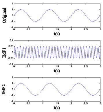
(a)

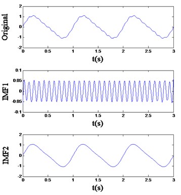
(b)

The most fundamental reason causing the mode mixing is the local extremum selection. One major procedure during the EMD process is calculating the upper and lower envelopes based on the local extremum, and it can be noticed that the amount and the location of the local extremum decides the main frequency components of the current IMF directly. Whether two components can be separated depends on the information of the local extremum. When the frequencies of two components are close, or the amplitude of the higher frequency component is low, the higher frequency component may not generate the local extremum reflecting the real frequency distribution and is hardly to decompose. As is shown in Fig. 1(b), IMF2 contains two components $c_1$ and $c_2$ with close frequencies 1 and 2 Hz, and the amplitude of $c_2$ is much lower, thus $c_1$ only influences the location of the local extremum, but cannot generate new local extremum, and they haven’t been separated.

To eliminate the mode mixing, differential algorithm is introduced into EMD. Theoretically, the differential signal has such properties: (1) it won’t change the frequencies of all the components; (2) it will increase the amplitude of component according to its frequency. It is noteworthy that the amplitude increase is linearly related to the frequency of the component, and according to the previous discussions, such properties are very helpful for improving the EMD. The higher frequency component with low amplitude will be strengthened in the differential signal, and may be able to generate new local extremum. The example above is utilized again to demonstrate the effectiveness of the differential EMD. First, the differential signals of $x_1$ and $x_2$ are calculated by central difference as follows:

where $\mathrm{\Delta }t$ presents a small increments of $t$, and then, the feature extraction process is carried out with the differential signals.

The result is shown in Fig. 2 and Table 2. Although an undesirable fake IMF appears in Fig. 2(b), the actual components implied in the differential signal of $x_2$ are decomposed into three IMFs effectively, and extracted feature vectors listed in Table 2 can be noticed to have high separability. Additionally, when the EMD result of the 1st-order differential signal still cannot separate the different frequency components, the 2nd-order and higher-order differential signals could be utilized:

Fig. 2The differential EMD result of the signal (a) x1 and (b) x2

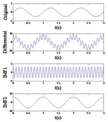
a)

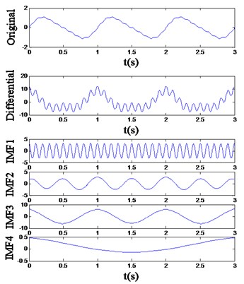
b)

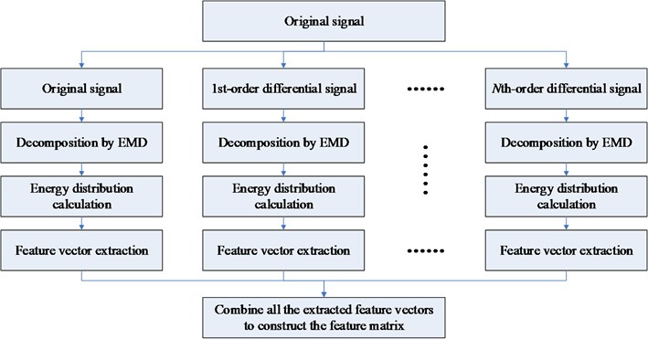
Based on the above studies, a novel Multi-Differential EMD (MDEMD) method is proposed to improve the effectiveness of the signal decomposition and feature extraction by combining the energy distribution characteristics of multi-order differential signals, and the flow chart of MDEMD is shown in Fig. 3. Multi-order differential signals are obtained, and the energy distribution features of these signals are extracted respectively. To represent the signal more comprehensively, all the extracted feature vectors are combined to construct the feature matrix. During the MDEMD process, the higher order is chosen, the more frequency information could be obtained, but the high order differential operation may lead to serious signal distortion. Therefore, the max order of multi-order differential signal $N$ should be decided by the complexity of the investigated signal.

Fig. 3The flow chart of MDEMD

3.1. Simulation signals

In this section, artificial signals are constructed to simulate the vibration signals of rotating machinery, and the simulation experiment is implemented to verify the superiority of the proposed MDEMD method. A set of signal components are defined in Eq. 4, and a certain combination of them can simulate the vibration response of the corresponding fault [18].

where $e_1\left(t\right)$ is a sinusoidal signal with the frequency of 60 Hz representing the 1$X$ component, $e_2\left(t\right)$ is an intra-wave modulated signal representing the $2X$ harmonic component, $e_3\left(t\right)$ and $e_4\left(t\right)$ are both sinusoidal signals representing the $4X$ and $6X$ harmonic components, and $e_5\left(t\right)$ is the noise signal. Previous researches have found that the $1X$ vibration is often caused by mass unbalance, and the excitation source of $2X$ vibration harmonic is usually misalignment, while the $4X$ and $6X$ vibration harmonic components constantly appear in the response of rubbing fault. In the simulation experiment, four classes of signals with different combinations of $e_1\left(t\right)-e_5\left(t\right)$ are established as follows:

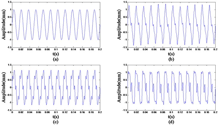
where $A$ is a random number in the range of [0.3, 0.4], $B$ is a random number in the range of [0.28, 0.32], and $C$ is a random number in the range of [0.09, 0.11]. Forty samples for each class are produced with different $A$,$B$, $C$, 25 of which are training samples and the other are testing samples. Fig. 4 gives a set of examples of the four classes.

Fig. 4Examples of the four classes: (a) x1, (b) x2, (c) x3 and (d) x4

3.2. Signal decomposing and feature extraction analysis

In the simulation experiment, the max-order of MDEMD is set to 2, and EMD is applied to the original and multi-order differential signals. As the amplitude of signal would change after the differential operation, in order to make the extracted energy distribution more convincing, the differential signal is divided by a determined factor equals to 120π, so that the amplitude of $1X$ component would keep invariant. The main IMFs obtained by EMD of the example signals are respectively shown in Fig. 5 to 7.

Fig. 5The decomposition result of the original signals

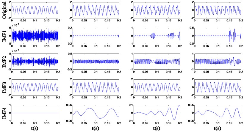
Fig. 6The decomposition result of the 1-order differential signals (1-ODS)

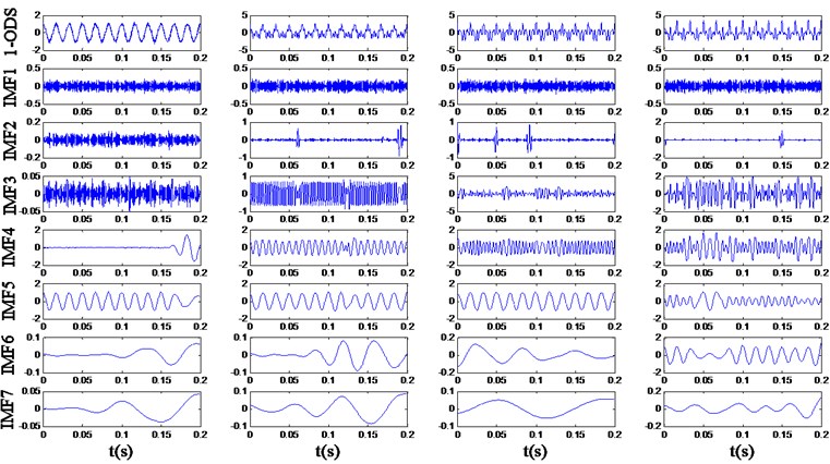
Fig. 7The decomposition result of the 2-order differential signals (2-ODS)

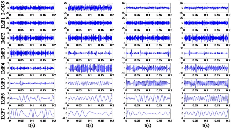
In Fig. 5 it is revealed that multiple frequency components contained in the simulation samples cannot be decomposed sufficiently by EMD and the mode mixing exists evidently. For example, the IMF3 of signal $x_2\left(t\right)$ and $x_4\left(t\right)$ contains $1X$ and $2X$ components, and the IMF2 of $x_1\left(t\right)$ contains 4$X$ and $6X$ harmonic components. In Fig. 6 and 7, the amplitude of higher frequency components rises more obviously through the differential process, and the influence of noise signals becomes more serious. However, although the smoothness of the signals decreases, the multiple frequency components implied in the multi-order differential signals can be decomposed more sufficiently.

Based on decomposition results, the feature matrixes of energy distribution are extracted and parts of them are listed in Table 3. Through comparison of the feature vectors extracted from multi-order differential signals, it is revealed that the energy distributions of four original signals are quite similar to each other, while the energy distributions of 1- and 2-order differential signals have quite big differences.

To verify the separability of the extracted features, Support Vector Machine (SVM), which is a common pattern recognition method based on the structural risk minimization (SRM) principle [27], is applied to identify the four classes of simulation signals with the energy distribution characteristics respectively obtained by the original EMD, 1- and 2-order MDEMD. The identification results are summarized in Table 4. By the original EMD method, the identification rates of the four classes are quite different and the average identification rates of training and testing samples are respectively 67.7 and 65.3 %, which are too low for the signal identification. By the 1-order MDEMD, all the identification rates are significantly improved, and the average identification rates rise to 93.9 and 94.2 %. By the 2-order MDEMD, the accuracy is further improved, and the identification rates of three classes have reached 100 %. The simulation experimental result verifies the separebility of the extracted features and demonstrates that the proposed MDEMD method is suitable for signal identification.

4.1. Data collection

Rolling element bearings are the major part of most rotating machineries, and detecting and diagnosing the existence and severity of bearing faults is significant to prevent the rotating mechanical system from fatal breakdowns. In this section, the proposed MDEMD method is applied to feature extraction and fault diagnosis for rolling element bearings.

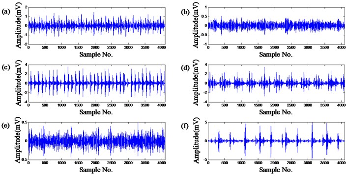
Part of the bearings vibration dataset collected by K. A. Loparo [28] is used in this paper. Three faults including outer race fault, inner race fault and ball fault, with the same defect sizes of 0.007 or 0.021 in, were respectively introduced into the drive-end bearing of the motor, which were tested under four different loads, 0, 1, 2 and 3 hp and the vibration data was collected at 12000 samples/s and 24000 samples/s by the installed sensors. In this paper, the vibration data collected at 12000 samples/s under 0 hp load with the defect sizes of 0.007 or 0.021 in was utilized and divided into 100 sub-signals with 4096 data points for each group. The produced 6 classes of samples covering 6 types of faults are listed in Table 5, and their time responses are illustrated in Fig. 8.

Fig. 8Time series of fault signals: (a) ball fault with 0.007 in; (b) inner race fault with 0.007 in; (c) outer race fault with 0.007 in; (d) ball fault with 0.021 in; (e) inner race fault with 0.021 in; (f) outer race fault with 0.021 in

4.2. Feature extraction and fault diagnosis

Based on the theories above, the energy distribution characteristics of all the samples are extracted from the original and multi-order differential signals respectively, and the length of the extracted feature vectors is set to 10 containing 1 $ET$ and 9 $EPs$. After feature extraction, the obtained feature matrixes were scaled to be in [0, 1].

The fault diagnosis experiments were carried out with the fault features respectively extracted by the original EMD, 1- and 2-order MDEMD, and half of the samples for each class were randomly selected as training data leaving the rest as testing data. Furthermore, the four most common classifiers including k-Nearest Neighbor algorithm (kNN), Radial Basis Function (RBF) Neural Network, Support Vector Machine (SVM) and Probabilistic Neural Network (PNN) were applied to identify the 6 classes of faults, and the experiment of each method was repeated for 30 times.

Table 6 shows the comparison results of different diagnostic methods, and the identification rates of training and testing samples are reported respectively. It is clear that, the testing accuracy of 1-order MDEMD is much higher than the original EMD and reaches to more than 98.70 %, while the identification rate of 2-order MDEMD is further increased to more than 99 %. It is also noticed that the identification accuracies of different classifiers varied in a small range. The minimum testing accuracy by using original EMD is 92.11 % for RBF while the maximum is 95.68 % for PNN, and the variance is 3.57 %. By using 1-order MDEMD, the minimum and maximum testing accuracies are respectively 98.70 and 99.33 % corresponding to RBF and PNN, and the variance deduced to only 0.63 %. Especially, by utilizing 2-order MDEMD the lowest accuracy is 99.04 % for kNN, and the identification rates of SVM and PNN are nearly 100 %. Therefore the effectiveness and universality of the proposed MDEMD are demonstrated.

Meanwhile, it is noteworthy that the higher order for MDEMD would produce lager feature matrix, and the time consumption would increase accompanied with the accuracy, thus, the selection of the proper order depends on the balance between the requirements of the accuracy and efficiency. For the fault diagnosis of rotating machinery, the recommended max order is 2. In summary, the comparison results reflect that MDEMD can stably extract the fault features with high separabilities and the fault diagnosis can be completed with satisfactory accuracy by using these fault features. It is feasible for fault diagnosis of rotating machinery.