Rotor fault classification technique and precision analysis with kernel principal component analysis and multi-support vector machines

1. Introduction

With the increasing complexity of structural forms of rotating machinery equipment and increasing running speed, the damage of components has been increasing significantly. Monitoring technology can provide effective warning information in the initial stage of fault to reduce the losses [1]. As the monitoring process is needed to measure many variables, there is a correlation between different variables, and if many correlative variables can be reduced to a few independent variables, which removes the redundant information obtained in the monitoring process [2], then we can find the root cause of fault from the remaining independent variables.

Now the most frequently used variable dimension reduction methods are all linear dimension-reduction methods, assuming that there is a linear correlation between variables in each process, and then the adopted dimensionality reduction and extraction of independent variables can realize the process monitoring and diagnosis [3]. For some high-speed rotating machinery such as aero-engine, the existence of many strong nonlinear excitation sources such as oil-film force and flow induced force in high-speed rotor system will cause many nonlinear features of rotor system. When a fault occurs in a rotor system such as the occurrence of rub-impact, surge, imbalance, and other faults, as well as the coupling faults, nonlinear problems, will become more prominent [4], so that it is necessary to use nonlinear methods to perform monitoring and analysis on system.

Kernel Principal Component Analysis (KPCA) feature extraction is more suitable for extracting nonlinear features in data in nonlinear fault feature extraction [5]. Support Vector Machine can achieve good classification results in case of a few training samples [6], and it has a strong generalization and anti-interference ability, which can demonstrate a unique advantage in solving classification problems of a small sample.

A vibration fault diagnosis approach for aero-engine based on Kernel Principal Component Analysis feature extraction and Support Vector Machines (SVM) classifiers is proposed in this paper, and this method takes advantage of the nonlinear feature extraction capability of KPCA to construct an eigenvector and a good classification, with learning and generalization for small samples of Support Vector Machine, which solves problems of small samples and nonlinear mode recognition in fault diagnosis of aero-engine test cell and achieves accurate state recognition of equipment. The test result for test cell shows that this method is feasible.

2. KPCA feature extraction

Fault diagnosis changes a system into a fault mode according to a set of measured eigenvector reflecting the working state of system and it is a mode classification problem. Vibration fault diagnosis process specifically includes three major steps: vibration signal acquisition, feature information extraction, and state classification recognition, in which feature information extraction is the key to fault diagnosis [7].

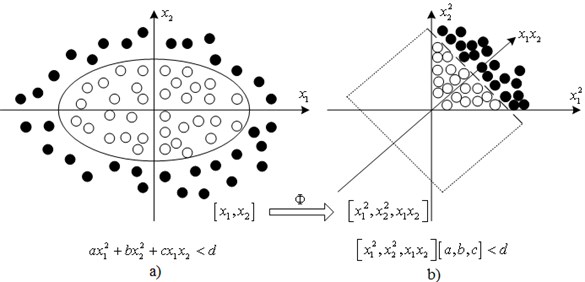
If linear inseparability, as shown in Fig. 1(a), exists in different types of the original data, then it can be asserted that the linear transform is unable to fundamentally change their linear inseparability, and also cannot turn these data into those that can be linearly separated, as shown in Fig. 1(b). Fig. 1 vividly demonstrates the role of nonlinear transform in strengthening the linear inseparability between different data.

As shown in Fig. 1, solid points and hollow points in the 2D data space represent the linear inseparability of two types of data, respectively, i.e. no straight line can be found to correctly separate them. While applying these data into a 3D space, we can find a plane to completely apart the two types.

Fig. 1Schematic diagram for nonlinear transformation to transfer the linear undetachable data into detachable data: a) inseparable data, b) separable data

Principles of KPCA Feature Extraction: In this method, a pre-selected set of nonlinear mapping can map the input data to a high dimensional feature space to make the input data have a better separability and choosing different kernel functions can get different nonlinear features. KPCA can achieve the transformation from input space to feature space through the nonlinear mapping $\mathrm{\Phi }$, and then performs linear PCA on the mapped data, so it can achieve a strong nonlinear processing ability.

For the $M$ samples in input space $x_k(k=\mathrm{1,2},\cdots ,M)$, $x_k\in R^N$, assuming $\sum _{k=1}^M{x}_k=0$, and then its covariance matrix was $C=\frac{1}{M}\sum _{j=1}^M{x}_j{x}_j^T$.

With general PCA method, an eigenvalue can be obtained with large contribution rate and its corresponding eigenvector by solving the characteristic equation $\lambda \nu =C\nu$.

Nonlinear mapping function $\mathrm{\Phi }$ is introduced to change the sample points $x_1,x_2,\dots ,x_M$ in the input space into sample points $\mathrm{\Phi }\left(x_1\right),\mathrm{\Phi }\left(x_2\right),\dots ,\mathrm{\Phi }\left(x_M\right)$ in the feature space, and assumed that:

Thus the covariance matrix in feature space $F$ is:

Therefore, the PCA in feature space is used to solve the eigenvalue $\lambda$ and the eigenvector $V\in F\backslash \left\{0\right\}$ in equation $\lambda \nu =\stackrel{-}{C}\nu$, and then there was:

It can be noted that $\nu$ in the above formula can be expressed by $\mathrm{\Phi }\left(x_i\right)(i=\mathrm{1,2},\cdots ,M)$ in a linear way that is:

It was available from the above formulas (2)-(4) that:

Define the $M\times M$ matrix $K$, $K_{ij}=\mathrm{\Phi }\left(x_i\right)·\mathrm{\Phi }\left(x_j\right)$.

Equation (4) can be simplified as:

This obvious satisfied:

So it absolutely satisfied Equation (6). By solving the Equation (7), the required eigenvalues and eigenvectors can be obtained. The projection of test samples on vector $V^k$ of space $F$ is:

All equations mentioned above are derived under the premise of the mapping data mean is zero, and that is to say Equation (1) is feasible, if not feasible in some cases, $k$ in Equation (7) can be replaced by $\tilde{K}$:

where $1_{ij}=1$ (for all $i$ and $j$).

Steps of KPCA Feature Extraction: Fault feature extraction steps are as follows:

(1) Standardize fault samples and eliminated the impact of nonstandard mode data to generate training matrix $X$.

(2) Utilize formula $K_{ij}=\mathrm{\Phi }\left(x_i\right)·\mathrm{\Phi }\left(x_j\right)$ to calculate the corresponding nuclear matrix $K$.

(3) Solve the characteristic Equation (7) to obtain the required eigenvalues and eigenvectors.

(4) Utilize the Equation (8) to calculate the projections on eigenvectors of all training samples, which are regarded as input eigenvectors of Multi-Classification Support Vector Machine.

3. Fault classification recognition algorithms

After feature extraction, the signal can retain most of fault information. What kind of fault, however, abnormal signal samples belong to is a problem with pattern classification recognition and the generalization ability and outreach capacity of Support Vector Machine algorithm can solve the classification recognition problems of small samples. This paper adopts Least Square-Support Vector Machine (LS-SVM) algorithm to solve the classification mode of fault diagnosis [8, 9].

SVM can get a fine classification effect with condition that the training sample is small. It overcomes some defects of the neural network learning method, such as the network structure is hard to be determined and local minimal points may exist. As well, it has strong ability in generalization and anti-interference, and shows unique advantages when classifying small samples.

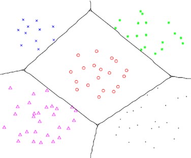
Following the principle of structural risk minimization, SVM is to make a balance between the precision of the given data and the complexity of the approximating function, and to achieve the minimization of the expected risks by minimizing both empirical risks and confidence interval. Based on the training samples, a judging criterion can be defined to minimize errors and losses that caused in process of classifying the objects. Fig. 2 shows the classification results.

Fig. 2Diagram of SVM classification and recognition

This kind of algorithm has advantages of simple algorithm and fast computational speed, as well as its training is completed by the following formula:

The constraint condition is $y_i{(W}^{T}g\left(x_i\right)+b)=1-{\epsilon }_i$, where $i=1,\dots ,M$; $y=\{+1,-1\}$; $W$ is the weight vector; $g\left(x\right)$ is a function that maps $X$ from the input space to the feature space; $\xi$ is the relaxation factor of $x_i$; $C$ is the boundary coefficient. Lagrange multiplier ${\alpha }_i$ is used to turn the above equation into an unconstrained objective function:

Perform the partial derivative on $W$, $b$, $\xi$ over Equation (11) to zero, the following optimal conditions can be obtained:

Substitute Equation (12) into Equation (14), then the results and Equation (13) can be shown in matrix form:

In this formula, $I={\left(1,\dots ,1\right)}^T$ is an $M$-dimensional vector $y={\left(y_1,\dots ,y_M\right)}^T$.

Solved matrix (15), $\alpha$ and $b$ can be obtained, then:

Least Square-Support Vector Machine (LS-SVM) turns the inequality constraints into equality constraints and its training process then is changed from solving the quadratic programming problem into solving linear equations, thus, simplifies the complexity of computation.

The structure of multi-classification Least Square-Support Vector Machine used to identify four working states of test cell is shown in Fig. 3.

In this algorithm, $m-1$ out of $m$ types are considered as one class, while the left type is considered as another class. In this way the first two-class classifier can be established. Next, select $(m-1)-1$ from the $m-1$ types as one class and the left as another to establish the second two-class classifier. The rest types are treated in the same manner till final classifier of the last two types is established. For $m$ types, a total of $m-1$ classifiers are needed. Such a classification method can lead to a small number of both classifiers and training samples, and thus can improve the speeds of training and identifying.

It is needed to establish four two-classification Support Vector Machine, and there is no existence of non-recognition domain in this type of multi-classification classifier, the less repeated training samples, and the fast training and recognition speed.

Fig. 3Flow chart of multi-SVM classification algorithm

4. Simulation application research

Aero-engine is an extremely complex nonlinear time-varying system that the main structure of aero-engine includes three concentric rotors and each rotor is connected by its own gas compressor and turbine through an axis and respectively rotates at different speed. There are usually 37 kinds of common faults and 28 corresponding variables in rotor system. Relationship between fault symptoms and fault reasons of rotor is not one to one mapping, but the relationship of one-to-many and many-to-one, and it is impossible to find a determinate relationship to diagnose faults of engine system.

The specific implementation steps of vibration fault classification approach for aero-engine based on KPCA mode and Support Vector Machines proposed in this paper are shown in Fig. 4.

Fig. 4Aero-engine vibration fault classification flow chart

Data are collected from certain type of engines at engine repair shop in Aircraft Maintenance Engineering Co., Ltd and data are collected when engine test cells simulating different faults.In order to establish fault classification mode based on KPCA and multi-classification SVM, a process monitoring on three kinds of common faults is conducted. First, the vibration data of normal state, fault of pedestal looseness, crack of oil tube, and turbine blade damage are collected, repectively, and some data are shown in Table 1.

For each type of work state, six sensor data of system for feature extraction are selected: exhaust gas temperature EGT (°C), fuel flow FF (kg/hr/daN), lubricating oil consumption WF (L/h), engine pressure ratio EPR, low-pressure rotor N1 (rpm), and low-pressure vibration V1 (IPS). Each working state performs 120 times of samplings at a certain sampling frequency and a total of 480 sampling data was obtained. Part of the monitoring results are shown in Fig. 5.

Fig. 5Three faults speed up-down monitoring process curve

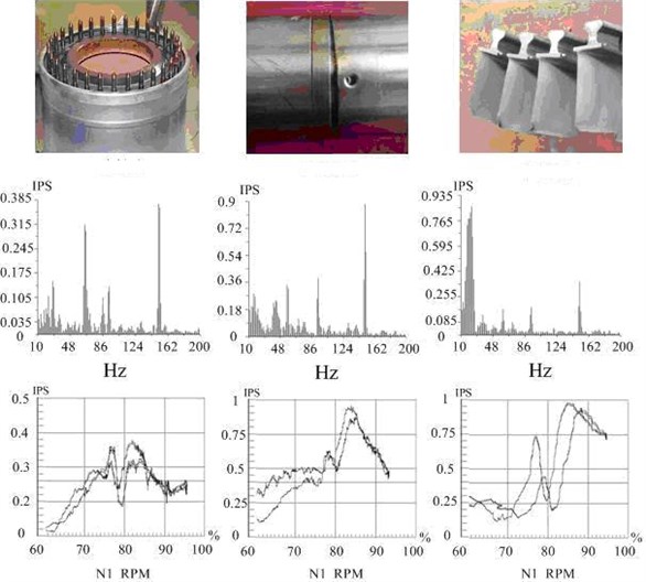
Normalization on 3 kinds of faults is performed and 6 types of data are collected from the sensors in the interval [0, 1]. 20 samples for 3 kinds of faults are collected and EGT, FF, V1, and N1 as the projection direction are chosen, thus, the projection drawing is shown in Fig. 6.

Fig. 6Two dimensional projection of three faults sample data: Pedestal looseness, Crack of oil tube, Turbine blade damage

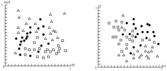
The figure showed that the situation of sample data of three kinds of faults mixed together is linearly inseparable.

To verify the fault features extraction of KPCA and classification effect of SVM, test steps are as follows:

(1) Arrange the six collected data by row into a one-dimensional array to represent one sample, and then all samples constitute the sample matrix A480×6 with each row representing a sample.

(2) Take 80 groups of data of each work state as training samples, and make use of KPCA to extract the principal components of sample matrix and extract the eigenvector of each sample to get the eigenvector set.

(3) Make use of the set of eigenvector as shown in Fig. 6, then input Least Squares Support Vector Machines to conduct training.

(4) Perform verification with the remaining 40 groups of samples. First extract the principal components projection for validating samples obtained by eigenvector and then input SVM using the output results to perform fault classification.

The classification accuracy of SVM mode have something to do with some influencing factors such as the type of kernel function, the penalty parameter $c$, and the kernel function parameter $g$. The commonly used kernel functions are linear kernel function, polynomial kernel function, radial basis function, two-sensor kernel function and so on.If the primary penalty parameter $c$ is 2, and 1 for the kernel function parameter $g$, the contrast for predicting classification accuracy of test set is shown in Table 2.

As can be seen from the table, the classification accuracy of radial basis function is relatively high after a number of experimental and theoretical analysis for high-speed rotor with prominent nonlinear dynamic characteristics such as aero-engine, and the classification predicting accuracy is higher than other kernel functions when using RBF kernel function, so this paper carries out analysis on RBF kernel function.

Table 2 also shows that, due to the influence of parameters values $c$ and $g$, the classification accuracy of RBF kernel function is not too high. That is because the classification accuracy is not only affected by these three kinds of factors, but also some factors will promote and constrain each other, thus affecting performance, and the overall effect is much larger than the impact of individual factor. Therefore, in the choices of kernel function, penalty parameter $c$, and kernel function parameter $g$, the influence of interaction of three kinds of factors on the system’s identification accuracy should be considered.

A multi-group cross-validation ($K-CV)$ idea is adopted to get the optimized $c$ and $g$ through optimization. The specific method is to divide the initial data into $K$ groups, the data of each subset can be regarded as validation set at a time, and the remaining data of $K-1$ subsets is regarded as the training set, thus getting $K$ modes. Then take the classification accuracy’s average of final validation set of those $K$ modes as the performance indicator of classifier in $K-CV$. The $K-CV$ method can effectively avoid the occurrence of state of over fitting and under fitting. As for the optimizing classification procedure of Support Vector Machine based on MATLAB platform design, graph’s $x$-axis corresponds to the value of $c$ with base 2 logarithm, $y$-axis corresponds to the value of $g$ with base 2 logarithm, and the contour line represents the accuracy of $K-CV$ method with certain $c$ and $g$. It can be seen from the figure that $c$ can be reduced to the range of 2^-2~2⁴, while the range of $g$ can be reduced to 2^-4~2⁴, so $c$ range is 2^-2, 2^-1.5,…, 2⁴, $g$ range is 2^-4, 2^-3.5,…, 2⁴, and the display interval changes of accuracy in the final parameters results map is set to 0.9. The best values of $c$ and $g$ in the optimization process can be obtained from the contour map whose test error rate changes with parameters and the 3D view is in Fig. 7, when $K=3$, the optimal parameter $c=$1.5324 and $g=$1.6572.

If several groups of $c$ and $g$ are corresponding to the highest validation classification accuracy, it is good to select the searched first groups $c$ and $g$ as the best parameters to avoid the over high $c$ leading to the state of over-fitting. That is to say that the classification accuracy of training set is very high while the classification accuracy of test set is very low (lowering the generalization ability of classifiers), so the smaller penalty parameter $c$ satisfies all the pairs of $c$ and $g$ in the highest validation classification accuracy, which is a better choice.

Fig. 7Contour map and 3D view of classification accuracy changing with parameters c and g

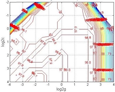
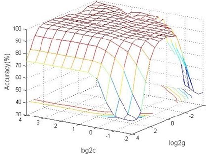
Fig. 8 shows classification results of some samples after KPCA feature extraction on 3 kinds of fault data using radial basis function and Least Squares Support Vector Machine classification method. Specific function value of a classifier is related to the samples, i.e. different samples are in need of different classifiers. The classifier functions are automatically given by MATLAB program. Combine these three classifiers according to Fig. 3. Such a multi-fault classifier is then able to separate three different types of faults. The classification facets of different types of samples are decided by the support vectors.

Fig. 8SVM classification facet of three faults model: Normal State, Pedestal Looseness, Crack of Oil Tube, Turbine Blade Damage

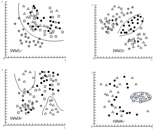
It can be seen from the figure that after the KPCA feature extraction, different faults can achieve a clearer classification by SVM.

The following table is used to show the selection of KPCA-SVM method, PCA-SVM, neural network, and SVM method based on fault feature sample, and it is a contrast based on the data classification of fault modes of normal state, pedestal looseness, vibration and crack of oil tube, and turbine blade damage (120 groups for each mode). It can be seen from Table 3 that the KPCA classification method selected based on the features of fault samples can improve the classification accuracy in the condition of guaranteeing the arithmetic speed, which ahs a better performance than other classification methods.

5. Conclusions

Combining the Kernel Principal Component Analysis extraction technology and Support Vector Machine and then applying them in the classification of aero-engine fault diagnosis mode, its performance is superior to many existing methods. The diagnostic accuracy is higher for small samples, but the diagnosis speed is faster for high-dimensional samples.

The parameters in testing modes of Support Vector Machine have a larger influence on detecting accuracy, such as penalty parameter and kernel function that can affect the classification performance of Support Vector Machine. Although these parameters can be determined by a large number of tests and be obtained using cross-examination, there is still no practical universal programs and lacks of theoretical guidance for parameters, so how to set these parameters to allow for better performance of SVM is a worthy research topic.

References

-
M. Sarvi, M. Sedighizadeh, A. A. Bagheri TTC enhancement through optimal location of facts devices using particle swarm optimization. International Review of Electrical Engineering, Vol. 6, Issue 1, 2011, p. 324-331.
Stappenbelt Brad Vortex-induced motion of nonlinear compliant low aspect ratio cylindrical systems. International Journal of Offshore and Polar Engineering, Vol. 21, Issue 4, 2011, p. 280-286.
Mamandi Ahmad, Kargarnovin Mohammad H. Dynamic analysis of an inclined Timoshenko beam traveled by successive moving masses/forces with inclusion of geometric nonlinearities. Acta Mechanica, Vol. 218, Issue 1-2, 2011, p. 9-29.
Xiangyang Jin, Xiangyi Guan, Lili Zhao Spectral analysis and independent component separation for aero-engine rotor vibration. International Review on Computers and Software, Vol. 7, Issue 5, 2012, p. 2740-2744.
S. Doughty Transfer matrix eigen solutions for damped torsional system. Journal of Vibration and Acoustics, Vol. 107, Issue 1, 1985, p. 128-132.
Zhu Ning, Feng Zhigang, Wang Qi Fault diagnosis of rocket engine ground testing bed based on KPCA and SVM. Journal of Harbin Institute of Technology, Vol. 41, Issue 3, p. 81-84.
Yuan Shengfa, Chu Fulei Support vector machines and its applications in machine fault diagnosis. Journal of Vibration and Shock, Vol. 26, Issue 11, 2007, p. 29-35.
T. H. Loutas, D. Roulias The combined use of vibration, acoustic emission and oil debris on-line monitoring towards a more effective condition monitoring of rotating machinery. Mechanical Systems and Signal Processing, Vol. 25, Issue 4, 2011, p. 1339-1352.
K. Umezawa, T. Suzuki, H. Houjoh Estimation of vibration of power transmission helical gears by means of performance diagrams on vibration. JSME International Journal, Vol. 31, Issue 4, 1998, p. 598-605.
About this article
This work was supported by the Scientific Research Fund of Heilongjiang Provincial Education Department (No. 12511124).