Abstract
A feature extraction method combined with variational mode decomposition (VMD) and kernel independent component analysis (KICA) is proposed to improve the fault feature extraction of vibration signal of rotary machinery. Firstly, VMD is used to decompose the single-channel vibration signal. Secondly, calculate the correlation coefficient between each component and the original signal. Finally, a new multidimensional observation signal is formed with high correlation components, and the fault signals will be extracted from the new observation signal by KICA. Compared with some typical fault feature extraction methods, the better performance of the proposed method is demonstrated by two experiments which are faulty rolling bearing experiment and a comprehensive experiment with faulty rolling bearing and faulty gear. Furthermore, an experiment of faulty rotary shaft verifies the effectiveness of this method. The results demonstrate that the proposed method is efficient for fault feature extraction of single-channel vibration signal of rotary machinery.
1. Introduction
Because of the progress of science and technology, rotary machinery is becoming more and more complex and precise in order to produce products of higher quality and higher precision. However, what follows is the complexity of its fault diagnosis. From the earliest dismantling to today's intelligent diagnosis, fault diagnosis has been studied for decades. From an empirical point of view, the fault of rotary machinery usually occurs in bearings, gears and rotary shafts. Therefore, many researchers are studying the fault diagnosis of these components by extracting fault features of vibration signals recently [1-3]. During the acquisition of vibration signals, due to a limited monitoring environment, it is often single-channel monitoring. In order to acquire more fault information of single-channel vibration signals of rotary machinery and improve the efficiency of fault diagnosis, many feature extraction methods have been proposed, some typical methods such as wavelets [4, 5], ensemble empirical mode decomposition (EEMD) + fast independent component analysis (FastICA) [6, 7] and so on. However, these methods have the problem that the extracted features sometimes are not obvious, and the noise energy is very high.
EEMD [8] is widely used in fault feature extraction, but it sometimes has mode mixing. Furthermore, it is affected by the sampling frequency, and the decomposition error sometimes is large. In order to avoid these problems, a new adaptive signal processing method, VMD [9, 10], is proposed. This method is used to search the optimal solution of the variational model by iterative search to determine the frequency center and bandwidth of each decomposition component. FastICA [11, 12] and KICA [13, 14] which are blind source separation (BSS) algorithms are often used in fault diagnosis recently. The vibration signal of large rotary machinery often mixes several signals and shows a strong nonlinear characteristic. Compared with FastICA, KICA has the advantage of extracting nonlinear signals. Therefore, this paper proposes a fault feature extraction method combining the advantage of VMD and KICA.
In this paper, a fault feature extraction method of single-channel vibration signal based on VMD-based KICA is proposed. The three experiments show that this method has a better performance than wavelets and EEMD + FastICA to extract the fault features of rotary machinery. The structure of this paper is as follows: the theory of VMD, KICA, correlation coefficient and evaluation index are introduced in Section 2. Section 3 gives a detailed procedure of the proposed method. The performance of the proposed method with faulty rolling bearing is evaluated in Section 4.1. In Section 4.2, the performance of the proposed method is evaluated by a comprehensive experiment with faulty rolling bearing and faulty gear. In Section 4.3, an experiment of faulty rotary shaft proves the effectiveness of the proposed method.
2. Theories
2.1. VMD
VMD is a new signal decomposition method, which is the process of solving the variational problem based on classical Wiener filter, Hilbert transform and frequency mixing. In this method, the frequency center and bandwidth of each decomposition component are determined by searching the optimal solution of the variational model, and the signal can be adaptively decomposed into a component with sparsity. It is assumed that each mode is a limited bandwidth with a central frequency, the central frequency and bandwidth are constantly updated during the decomposition process, and VMD is finding the mode function , with the smallest sum of estimation bandwidths, and the sum of the mode functions is the input signal . The bandwidth of each mode function is determined through the following steps:
(1) In order to obtain the analytic signal of the mode function, Hilbert transform is performed for each mode function , that is:
where is time, is impact function, is components.
(2) Modulate the spectrum of each mode to the corresponding baseband, that is:
where is the center frequency of .
(3) Estimate the bandwidth of each mode component. The corresponding constraint variational model expression is as follows:
In order to obtain the above constraint variational problems, the penalty factor of the quadratic term and the Lagrange multiplication operator are introduced. is a large enough positive number, which can guarantee the reconstruction precision of the signal under the presence of Gaussian noise. The Lagrange operator makes the constraint conditions strict, and the extended Lagrange expression is:
The above variational problem is obtained by using alternate direction method of multipliers (ADMM), and the saddle points of the extended Lagrange expression can be obtained by alternately updating , and . is the mode function at the th cycle, and is the center of the power spectrum of the current modal function. is the multiplication operator of the th cycle. The solution process of can be expressed as:
where . By using the Fourier isometric transformation, Eq. (5) can be transformed to the frequency domain and replaced with , and the result is transformed into the form of negative frequency interval integral. The solution of the optimization problem is:
According to the same process, get the center frequency update mode:
where is equivalent to the Wiener filtering of . The Fourier transform to , the actual part is .
The specific implementation process of the VMD method is as follows:
(1) Initialize mode function , center frequency , Lagrange multiplication operator, initial cycle times 0.
(2) Execute the cycle .
(3) Update , .
(4) Update . where is a time constant, usually taken as 0.
(5) Given discriminant accuracy 0, repeat the above steps until the iteration stop condition is satisfied:
2.2. KICA
The mathematical description of independent component analysis (ICA) is: , where is a vector of source signals, is a vector of M mixed signals, The mixing matrix is a × dimensional matrix, is noise vector. The meaning of ICA is that when the mixing matrix and source signals are unknown, we only determine the remove-mixing matrix based on the observed data, and the output is the estimation of source signals.
KICA is not a simple nucleation of ICA, but a new ICA method. The idea of kernel technology is to use nonlinear mapping , and map the nonlinear variable of original input space into a kernel feature space to linearize it, and then analyse the mapped data in this feature space. Thus, the linear blind source separation in the space is equivalent to nonlinear blind source separation in the original space. One of the important characteristics of this technology is that kernel function can be used instead of inner product between two vectors to realize nonlinear transformation without specific form being considered. The kernel function of radial basis function (RBF) is chosen here.
KICA is characterized by the use of nonlinear functions as a contrast function in reproducing kernel Hilbert space (RKHS), the signal is mapped from low-dimensional space to the high-dimensional space, and this method is used to find out the minimum value of contrast function in this space. This function has a certain correlation with mutual information and has better mathematical properties. Moreover, this function space is suitable for various source signals. Therefore, compared with traditional ICA, KICA has better flexibility and robustness.
The KICA’s contrast function is constructed by calculating the correlation of a set of random variables directly. Let be a real vector function space, for simple calculations, and are two unary random variables of space . Define the correlation coefficient of and as the maximum correlation coefficient between random variables and :
is also called a contrast function between random variables. Obviously, if and are independent, so, 0. If space is large enough and 0, and are also independent of each other. The procedure of KICA is as follows:
Input: Data vector , , …, and kernel function .
Step 1: Whiten data vector , , …, .
Step 2: Use Cholesky decomposition to find the Gram matrix (, , …, of original independent data, where ( is the remove-mixing matrix).
Step 3: Define be the maximum eigenvalue of Eq. (10):
Step 4: Minimize for .
Output: .
This algorithm keeps running repeatedly between Step 2 and Step 4 until the convergence condition is satisfied, so that the remove-mixing matrix can be obtained. According to , for a set of observed data , , …, , the original independent source signals can be estimated effectively through the remove-mixing matrix .
2.3. Correlation coefficient
The formula for the correlation coefficient of component signal to the source signal is as follows:
where is the mixed source signal. is the th component signal. and are the variance of signal and . is the covariance between the signal and .
2.4. Evaluation index
The fault signal extracted from the real signal generally contains some noise. In the power spectrum of the extracted fault signal, the power of the fault frequency is usually the highest, so other frequencies can be considered as noise. If the power of noise is very close to or even higher than the power of fault frequency, the fault type cannot be accurately determined. Therefore, in order to compare the extraction effect of each fault diagnosis method, this paper proposes an evaluation index :
where is the power of fault frequency. is the power of the noise of the highest amplitude. Therefore, the bigger the value of , the better the effect of the extraction.
3. Detailed procedure of the proposed method
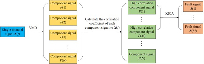
In this paper, a fault diagnosis method of rotary machinery based on VMD-based KICA is proposed. The procedure of the proposed method has been summarized in Fig. 1. The detailed procedure is described as follows:
Step 1: The collected single-channel signal is decomposed with VMD and each component signal can be obtained.
Step 2: Calculate the correlation coefficient of each component signal to . Then, choose high correlation component signals to form a new observation signal.
Step 3: Use KICA to extract the fault signals from the new observation signal.
Fig. 1The summarized procedure of the proposed method
4. Experiments
4.1. Faulty rolling bearing experiment
In order to verify the validity of the proposed method for faulty rolling bearing vibration signal, the test data from the bearing database of Case Western Reserve University are selected for analysis. The rolling bearing used in the test is SKF6205. The motor speed is 1800 rpm, that is, the rotation frequency 30 Hz. The sampling frequency 12000 Hz and the number of sampling points is 12000. The inner and outer rings of the rolling bearing are respectively machined with tiny pitting pits to simulate the fault of inner ring and outer ring. The fault frequency of inner ring can be expressed as:
The fault frequency of outer ring can be expressed as:
where is the number of roller, is the diameter of roller, is the pitch diameter of bearing, and is bearing contact angle. According to Eq. (13) and Eq. (14), 162 Hz and 107 Hz.
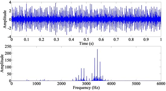
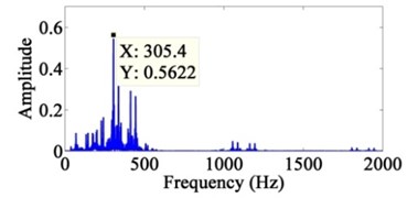
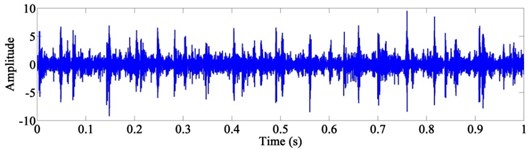
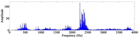
The time-domain waveform and power spectrum of single-channel vibration signal of inner ring fault and outer ring fault mixed are shown in Fig. 2.
The fault features of inner ring and outer ring cannot be found from time-domain waveform and power spectrum in Fig. 2. Therefore, so as to verify the high efficiency of the proposed method, the effect of feature extraction of wavelets, EEMD+FastICA and the proposed method are compared as follows.
Fig. 2The time-domain waveform and power spectrum of the observation signal
A. Wavelets.
In this method, the observation signal is decomposed with six-layer wavelet decomposition, and then the power spectrum of each component can be obtained. The result is shown in Fig. 3. and are not extracted, so the evaluation index can be considered as . Therefore, wavelets cannot extract the feature of fault signals of rolling bearing.
B. EEMD + FastICA.
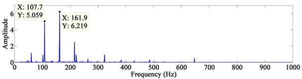
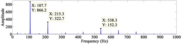
In this method, the observation signal is decomposed by EEMD first, and each intrinsic mode function (IMF) can be obtained. Then, calculate the correlation coefficient of each IMF to the observation signal. IMFs with high correlation coefficient were selected to reconstruct the new observation signal. Finally, the fault signals can be extracted by FastICA. The power spectrum of the extracted fault signals is shown in Fig. 4.
In Fig. 4(b), the frequency of 107.7 Hz which is very close to is extracted and its double frequency is also extracted. The frequency of 538.3 Hz is the noise of the highest amplitude. The frequency of 161.9 Hz which is very close to can be seen in Fig. 4(a), but the frequency of 107.7 Hz is also obvious, and it can be considered as noise now. Therefore, mode mixing occurs at this time. According to Eq. (12), 4.687, 0.229.
Fig. 3The power spectrum of the decomposed signals after wavelets: a) the sixth layer of low-frequency component, b) the sixth layer of high-frequency component, c) the fifth layer of high-frequency component, d) the fourth layer of high-frequency component
a)
b)
c)
d)
Fig. 4The power spectrum of the extracted signals after EEMD + FastICA
a)
b)
C. The proposed method.
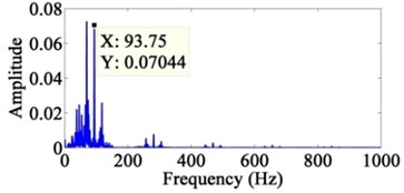
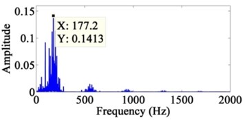
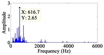
In this method, the observation signal is decomposed by VMD ( 4, 1000) first and each component signal can be obtained. Then, calculate the correlation coefficient of each component signal to the observation signal and their values are in Table 1. Component signals with high correlation coefficient (Threshold > 0.5) were selected to reconstruct the new observation signal. Finally, the fault signals can be extracted by KICA. The power spectrum of the extracted fault signals is shown in Fig. 5.
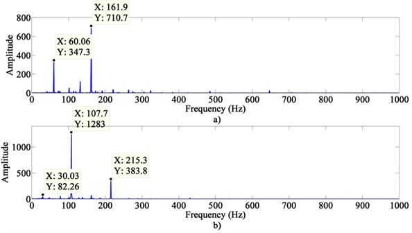
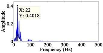
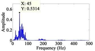
The frequency of 161.9 Hz which is very close to can be seen in Fig. 5(a). The frequency of 60.06 Hz is the noise of the highest amplitude. In Fig. 5(b), the frequency of 107.7 Hz which is very close to is extracted and its double frequency is also extracted. The frequency of 30.03 Hz is the noise of the highest amplitude. Furthermore, the fault features are very obvious. According to Eq. (12), 14.597, 1.046.
Table 1Correlation coefficient of each component signal
Serial number | Value |
i1 | 0.155 |
i2 | 0.193 |
i3 | 0.585 |
i4 | 0.801 |
Fig. 5The power spectrum of the extracted signals after VMD + KICA
The evaluation index of the three methods are in Table 2. The of the proposed method is much bigger than other two methods. Therefore, the proposed method has a better effect of extraction. The result proves that the proposed method is efficient to extract the features of single-channel vibration signal of rolling bearing with the fault of inner ring and outer ring mixed.
Table 2Evaluation index statistics
Evaluation index | ||
Method | ||
Wavelets | ||
EEMD + FastICA | 4.687 | 0.229 |
The proposed method | 14.597 | 1.046 |
4.2. Comprehensive experiment with faulty rolling bearing and faulty gear
The experimental device is shown in Fig. 6. The whole device is driven by a 550 W (220 V-50 Hz) AC motor and drives the shaft system with couplings. The shaft section between two bearing seats is equipped with a belt wheel, and the belt drives the active gear shaft of gear box. One acceleration transducer is installed vertically on the shell near the rolling bearing. There are two rolling bearings on the shaft system, and one of them is machined with tiny pitting pits on the outer ring to simulate the fault of outer ring. The sampling frequency 8192 Hz and the number of sampling points is 8192. The motor speed is 850 rpm, that is, the rotation frequency 14.2 Hz.
According to Eq. (14), 70 Hz. Destroy one tooth of the driving gear to simulate the fault of tooth breaking. The number of gear teeth 20. The number of the broken teeth 1. According to , the gear mesh frequency 283.3 Hz. When the gear is affected by broken tooth fault, the rotation frequency and its frequency multiplication will be the main features in frequency-domain, and the frequency will also exist. The time-domain waveform and power spectrum of single-channel mixed signal are shown in Fig. 7.
Fig. 6The experimental device
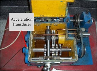
Fig. 7The time-domain waveform and power spectrum of the mixed signal
a)
b)
Fig. 8The power spectrum of the decomposed signals after wavelets: a) the seventh layer of low-frequency component, b) the seventh layer of high-frequency component, c) the sixth layer of high-frequency component, d) the fifth layer of high-frequency component
a)
b)
c)
d)
The fault features of outer ring and gear breaking cannot be found from time-domain waveform and power spectrum in Fig. 7. Therefore, the effect of feature extraction of wavelets, EEMD + FastICA and the proposed method are compared as follows:
A. Wavelets.
In this method, the mixed signal is decomposed with seven-layer wavelet decomposition, and then the power spectrum of each component can be obtained. The result is shown in Fig. 8. The fault features are not extracted, so the evaluation index can be considered as .
B. EEMD + FastICA.
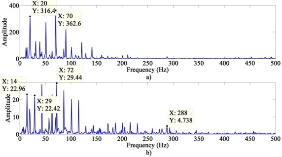
In this method, the mixed signal is decomposed by EEMD first, and each intrinsic mode function (IMF) can be obtained. Then, calculate the correlation coefficient of each IMF to the mixed signal. IMFs with high correlation coefficient were selected to reconstruct the new observation signal. Finally, the fault signals can be extracted by FastICA. The power spectrum of the extracted fault signals is shown in Fig. 9.
The frequency of 70 Hz which is very close to can be seen in Fig. 9(a). The frequency of 20 Hz is the noise of the highest amplitude. In Fig. 9(b), the frequency of 14 Hz which is very close to and its double frequency are extracted, and the frequency is also extracted. The frequency of 72 Hz is the noise of the highest amplitude. According to Eq. (12), 0.146, –0.220.
Fig. 9The power spectrum of the extracted signals after EEMD + FastICA
C. The proposed method.
In this method, the mixed signal is decomposed by VMD ( 6, 1000) first and each component signal can be obtained. Then, calculate the correlation coefficient of each component signal to the mixed signal and their values are in Table 3. Component signals with high correlation coefficient (Threshold > 0.5) were selected to reconstruct the new observation signal. Finally, the fault signals can be extracted by KICA. The power spectrum of the extracted fault signals is shown in Fig. 10.
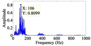
Fig. 10The power spectrum of the extracted signals after VMD + KICA
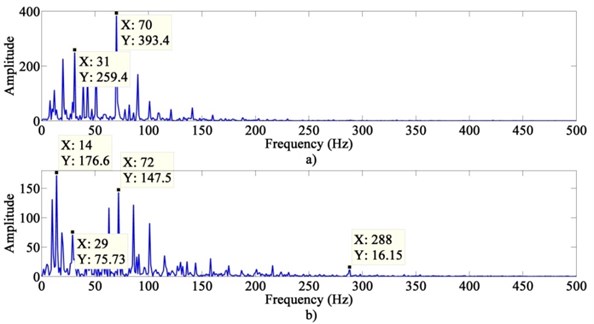
Table 3Correlation coefficient of each component signal
Serial number | Value |
i1 | 0.137 |
i2 | 0.150 |
i3 | 0.188 |
i4 | 0.606 |
i5 | 0.502 |
i6 | 0.091 |
The frequency of 70 Hz which is very close to can be seen in Fig. 10(a). The frequency of 31 Hz is the noise of the highest amplitude. In Fig. 10(b), the frequency of 14 Hz which is very close to and its double frequency are extracted, and the frequency is also extracted. The frequency of 72 Hz is the noise of the highest amplitude. Furthermore, the fault features are obvious. According to Eq. (12), 0.517, 0.197.
The evaluation index of the three methods are in Table 4. The of the proposed method is much bigger than other two methods. Therefore, the proposed method has a better effect of extraction. The results demonstrate that the proposed method is efficient to extract the fault features of single-channel vibration signal of complex machinery.
Table 4Evaluation index statistics
Evaluation index | ||
Method | ||
Wavelets | ||
EEMD + FastICA | 0.146 | –0.220 |
The proposed method | 0.517 | 0.197 |
4.3. Faulty rotary shaft experiment
A faulty rotary shaft experiment is applied to verify the effectiveness of the proposed method. The schematic diagram of test system is Fig. 11 and the test rig and signal acquisition system is shown in Fig. 12.
Fig. 11The schematic diagram of test system
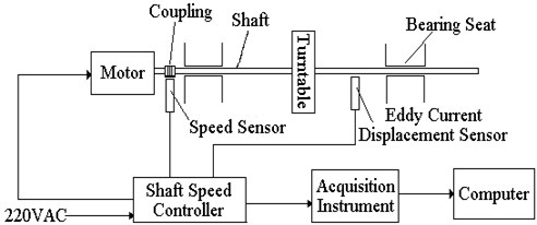
Fig. 12The test rig and signal acquisition system of faulty rotary shaft
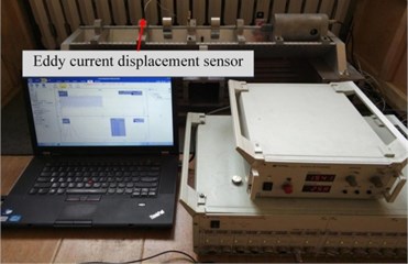
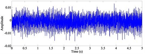
In this experiment, the artificial misalignment fault and rub-impact fault are created. Only one eddy current displacement sensor is used to collect the mixed vibration signal of faulty shaft. The sampling frequency is 1000 Hz and the number of sampling points is 5000. The motor speed is 2000 rpm, that is, the rotation frequency 33.3 Hz. According to experience, the feature of misalignment fault is that a higher amplitude of appears, even exceeding the amplitude of in frequency-domain. The feature of rub-impact fault is emerging 1/ of , where is equal to 2, 3, or 4. The time-domain waveform of the collected signal is shown in Fig. 13.
Fig. 13The time-domain waveform of the collected signal
In the proposed method, the collected signal is decomposed by VMD ( 4, 1000) first and each component signal can be obtained. Then, calculate the correlation coefficient of each component signal to the collected signal and their values are in Table 5. Component signals with high correlation coefficient (Threshold > 0.5) were selected to reconstruct the new observation signal. Finally, the fault signals can be extracted by KICA. The power spectrum of the extracted fault signals is shown in Fig. 14.
Table 5Correlation coefficient of each component signal
Serial number | Value |
i1 | 0.551 |
i2 | 0.579 |
i3 | 0.135 |
i4 | 0.133 |
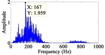
Fig. 14The power spectrum of the extracted signals after VMD + KICA
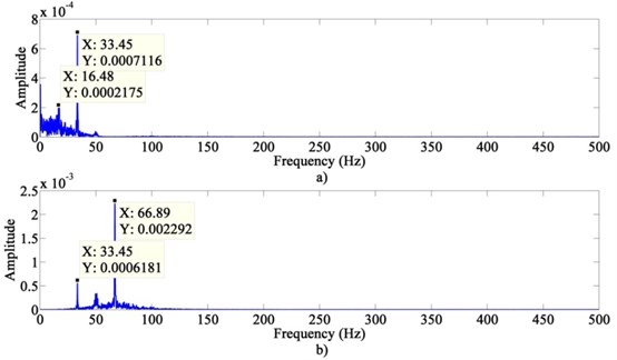
Both the frequency of 33.45 Hz and the frequency of 16.48 Hz which is equal to half of can be found in Fig. 14(a). It can be considered as the feature of rub-impact fault. In Fig. 14(b), the amplitude of 66.89 Hz is larger than 33.45 Hz, which can be considered as the feature of misalignment fault. Furthermore, the fault features are significantly obvious. It demonstrates that the proposed method has a good performance of the fault feature extraction of rotary shaft with the misalignment fault and rub-impact fault mixed.
5. Conclusions
The method of VMD-based KICA has been proposed to improve the fault feature extraction of single-channel vibration signal of rotary machinery in this paper. In the experiment of rolling bearing with the fault of inner ring and outer ring mixed, the evaluation index of the proposed method is much bigger than wavelets and EEMD+FastICA, it proves that the proposed method makes the fault features more obvious. In the comprehensive experiment with faulty rolling bearing and faulty gear, evaluation index demonstrates that the proposed method can clearly extract the fault feature of complex machinery. The experiment of faulty rotary shaft verifies the effectiveness of this method. Therefore, the proposed method is efficient for fault feature extraction of single-channel vibration signal of rotary machinery.
References
-
Medoued A., Mordjaoui M., Soufi Y.,Sayad D. Induction machine bearing fault diagnosis based on the axial vibration analytic signal. International Journal of Hydrogen Energy, Vol. 41, Issue 29, 2016, p. 12688-12695.
-
Zuber N., Bajrić R., Šostakov R. Gearbox faults identification using vibration signal analysis and artificial intelligence methods. Physiology and Behavior, Vol. 54, Issue 2, 2014, p. 407-409.
-
Harmouche J., Delpha C., Diallo D. Improved fault diagnosis of ball bearings based on the global spectrum of vibration signals. IEEE Transactions on Energy Conversion, Vol. 30, Issue 1, 2015, p. 376-383.
-
Yan R., Gao R. X., Chen X. Wavelets for fault diagnosis of rotary machines: A review with applications. Signal Processing, Vol. 96, Issue 5, 2014, p. 1-15.
-
Mishra C., Samantaray A. K., Chakraborty G. Rolling element bearing fault diagnosis under slow speed operation using wavelet de-noising. Measurement, Vol. 103, 2017, p. 77-86.
-
Jiang S. F., Chen Z. G., Shen Q. H., Wu M. H., Ma S. L. Damage detection and locating based on EEMD-Fast ICA. Journal of Vibration and Shock, Vol. 35, Issue 1, 2016, p. 203-209.
-
Zhao J., Jia R., Wu H. Extraction of vibration signal features based on FastICA-EEMD. Journal of Hydroelectric Engineering, Vol. 36, Issue 3, 2017, p. 63-70.
-
Xue X., Zhou J., Xu Y., Zhu W., Li C. An adaptively fast ensemble empirical mode decomposition method and its applications to rolling element bearing fault diagnosis. Mechanical Systems and Signal Processing, Vol. 62, 2015, p. 444-459.
-
Dragomiretskiy K., Zosso D. Variational mode decomposition. IEEE Transactions on Signal Processing, Vol. 62, Issue 3, 2014, p. 531-544.
-
Mohanty S., Gupta K. K., Raju K. S. Hurst based vibro-acoustic feature extraction of bearing using EMD and VMD. Measurement, Vol. 117, 2018, p. 200-220.
-
Dermoune A., Wei T. FastICA algorithm: five criteria for the optimal choice of the nonlinearity function. IEEE Transactions on Signal Processing, Vol. 61, Issue 8, 2013, p. 2078-2087.
-
Grueiro M. Q., Prieto-Moreno A., Santiago O. L. A procedure to configure the FastICA algorithm in fault diagnosis on industrial systems. Ingeniería Electrónica Automática Y Comunicaciones, Vol. 35, Issue 2, 2014, p. 73-89.
-
Hao T., Tang L. W., Tian G., Zhang Y. Fault diagnosis of gearbox based on KICA. Journal of Vibration and Shock, Vol. 28, Issue 5, 2009, p. 163-167.
-
Zhang Y., Du W., Li X. Observation and detection for a class of industrial systems. IEEE Transactions on Industrial Electronics, Vol. 64, Issue 8, 2017, p. 6724-6731.
Cited by
About this article

This research is subsidized by the Natural Science Foundation of China “Research on reliability theory and method of total fatigue life for large complex mechanical structures” (Grant No. U1708255).
