Pressure fluctuation identification of draft tube based on singular value decomposition and cascade correlation neural network

3.1. Cascade correlation neural network

Cascade correlation is a supervised learning algorithm for artificial neural networks which was developed by Fahlman and Lebiere [18]. It starts with a minimal network consisting only of an input and an output layer, then by minimizing the overall error of a network; it adds step by step new hidden units to the hidden layer to create a multi-layer structure, the method learns much faster than the usual learning algorithms.

It mainly consists of two key ideas: firstly, the cascade architecture, in which hidden units are joined to the architecture every time and is not altered after they have been joined in. Secondly, the learning method would generate and then install the new hidden units. We would try to magnify the magnitude of the cascade correlation between the output and the remainder of the error we are trying to evaluate.

We start on the first cycle, a single new hidden unit is generated and a weight connection from each input unit is given [19, 20]. The learning should be continued only if the error value does not meet the specific requirement, so a candidate node hidden unit is added to the network, but its output is not connected to the network, at this time, the weights of the candidate node can be trained while all the other weights in the network are frozen. During the candidate node training the goal is to maximize the value of correlation $C$ between the output of the candidate node and network output error:

where $y_p$ is the candidate’s output for the sample $p$, $e_{op}$ is the error at output node $o$ for the sample $p$, $\overline{y}$ and ${\overline{e}}_o$ are the mean values of the outputs and output errors over the all patterns of the training sample, the gradient ascent algorithm is usually used to obtain the maximization.

The second cycle gives the output of the new hidden unit a weight connection for each output unit. The entire set of connections to those from all input and hidden units would be trained through minimizing the sum squared error equation:

where $y_{op}$ and $t_{op}$ are the network output for pattern $p$ and the expected output for this pattern respectively.

3.2. Feature extraction

Feature extraction is to analyze the basic data and get the characteristics of data, in this paper, the pressure pulsation signal is decomposed by wavelet, the appropriate frequency band signal is chosen, the root mean square value of each frequency band is the recognition parameter, and the band of the RMS value is:

where $E_i$ is the RMS value in node $i$, $A_j$ is the discrete amplitude of reconstruction signal, $N_i$ is the number of data points to reconstruct the signal.

The flowchart of the CC neural network learning combined with singular value decomposition for the vibration signal of draft tube is given in Fig. 1.

4.1. Test procedure and measuring point layout

In order to get the hydraulic pressure fluctuation signal of the draft tube, the pressure pulsation test of the mixed flow turbine is carried on at turbine energy test stage in China institute of water resources and hydropower research, the main parameters of the model turbine: the wheel nominal diameter is 0.35 m, the blade number of the runner is 14, the height of the guide vane is 0.2 m, the distribution circle diameter of the guide vane is 1.18 m, the number of the fixed guide vane is 24, and the spiral angle is 350°.

Fig. 1The chart of vibration signal identification

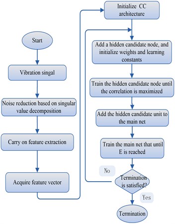
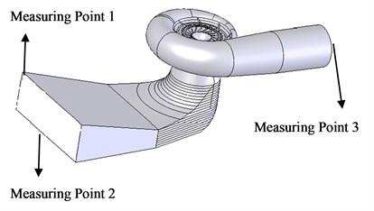
Fig. 2Measuring point layout

4.2. Data collection

Before the test, the pressure pulsation sensor is installed on the measuring point, the end face of the sensor must be flush with the port side of wall, after setting the calibration, the relationship between voltage and pressure is set up. In the experiment, the signals from the sensor are conveyed to the computer. The 69 signal data are obtained in each measuring point, the data length $N$ is 25600 from the collected vibration signals, the part data are as follows in Table 1.

4.3. Noise reduction and feature extraction

The noise reduction based on singular value decomposition is used to deal with the data, the analysis results are shown in the below figures, we can see from Fig. 3 that the noise of the original signal obtained has the bigger degree of inhibition, which is beneficial to the follow-up feature extraction. The collected signals in sample 1 and 2 are decomposed by the wavelet decomposition, the analysis results are shown in the below Fig. 4.

$t1=$[2.8076, 1.5926, 0.7937, 0.3440, 0.0865, 0.0215],

$t2=[$4.5107, 1.1953, 0.5801, 0.2964, 0.0961, 0.0601].

Fig. 3a) The original waveform of vibration signal, b) the waveform after noise reduction

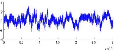
(a)

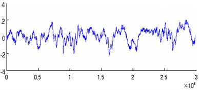
(b)

Fig. 4a) Low frequency and high frequency of 1-5 layers in sample 1, b) low frequency and high frequency of 1-5 layers in sample 2

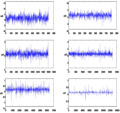
(a)

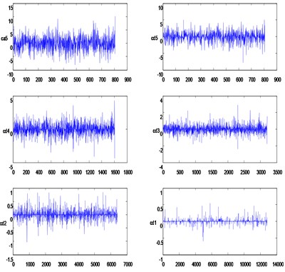
(b)

The signal information in each frequency band can be seen from above figures, the standard deviations of each frequency band for all samples are shown in Table 2.

4.4. The analysis of pressure pulsation based on cascade connection network

From the synthetic characteristic curve [21-23], we can get the pressure fluctuation value of corresponding samples, which are shown in Table 3. According to the pressure fluctuation value, the hydraulic pressure pulsation can be divided into three states including the normal state, the early vortex and the severe vortex. The corresponding value of the first state is between 1 % to 3 %, indicating that the pressure pulsation is lighter; the corresponding value of the second state is between 4 % to 5 %, indicating that the pressure fluctuation is bigger; the corresponding value of the third state is between 6 % to 8 %, indicating that the pressure pulsation is serious, the samples distributions are shown in Table 4.

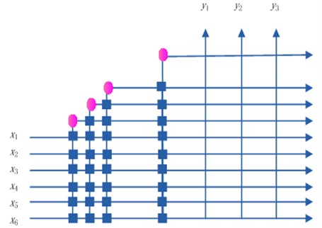
The 69 groups of feature vectors are as the input samples, the input node number of CC is six, and the output node number is three. After determining the number of the input and output, the adaptive learning based on the CC is applied to the model, the training results in 13 hidden neurons added to the actual network, finally the stable network model is 6-13-3 structure as shown in Fig. 5. Then the training the CC network is tested for accuracy and generalization using a testing set.

Fig. 5The network model based on CC

Six pressure pulsation points are taken from the comprehensive characteristic curve of the turbine as validation samples, and a comparison with BP neural network is made in order to evaluate the method properly. The BP network is trained using fast back-propagation method. Training parameters are set as follows: the learning rate is 0.02 and the momentum constant is 0.9. The weights and biases are initialized randomly. The BP network is trained with the same training samples, and the same test samples are used too in testing. The error is set as 0.001, 0.0003 and 0.0001 respectively. The results of the comparison between the two methods are shown in Table 5.

Compared with BP network, the result in Table 5 shows that the most evident characteristics of the proposed method are its robustness and less training time. If the number of hidden units of BP network is appropriate, it can improve its performance by reducing the error, but it can be seen that when the error is drop down from 0.001 to 0.0003, the error is down too. But when the error is small enough, due to the over-fitting, one cannot improve the result by reducing the error anymore. The test accuracy achieved with CC is 99.71 % using 13 hidden units, CC network has been shown to be capable of good generalization when it is applied to the pressure fluctuation identification of draft tube, the experiment with different numbers of hidden units is not necessary and the training time is 12.6 seconds less than that with standard BP networks with different hidden units, exhibiting good classification accuracy and rapid convergence speed.