Identification of a certain mechanism’s recoiling mass by limited memory least square method

Xu, Rui; Chen, Qiang; Yang, Guolai; Yan, Hao

Journal of Vibroengineering

Browse Journal

Submit article

Published: 15 February 2014

Check for updates

Identification of a certain mechanism’s recoiling mass by limited memory least square method

Rui Xu¹

Qiang Chen²

Guolai Yang³

Hao Yan⁴

^{1, 3}School of Mechanical Engineering, Nanjing University of Science and Technology, China

^{2, 4}Department of Control and System Engineering, Nanjing University, China

Corresponding Author:

Qiang Chen

Cite the article Download PDF

Downloads 1001

Abstract

This paper is concerned with the identification problem of a certain mechanism’s dynamic parameters in its operation. This mechanism can be simplified as three rigid body structure joined by a prismatic pair, a revolute pair and a fixed constraint. The unrestraint dynamic equations of the mechanism can be obtained by using multi-rigid-body theory. In order to acquire unknown dynamic parameters, such as displacement, velocity and acceleration, a field experiment was designed. Then by choosing limited memory least square method and using the experiment results, one mass of rigid body could be identified. Finally, the calculative mass was compared to the “real” mass which was consulted in the specification book of this mechanism. The whole process shows that the rigid dynamic model of this mechanism and the method of identification are both effective.

1. Introduction

The structure of machinery is becoming more and more complex. As a result that the mass matrix and the stiffness matrix of the whole system is also complex presenting time-varying. So, it’s difficult for researchers to describe the dynamic model of some machinery accurately.

At present, research field is mainly divided into two direction, forward problem and inverse problem. Based on mathematical model, forward problem is concerned with the structure’s dynamic response under different excitation. Q. Chen analyzed a certain mechanism dynamic response by using the wavelet transform method [1]. By means of multi-body transfer matrix method, X. Rui obtained the model function’s accurate expression [2]. Inverse problem, namely, dynamic parameter identification problem, uses some model class to find an equivalent model upon input and output. X. Liu, D. Jing and W. Zhuang provide many identifying methods of time-varying parameters in their papers [3-5]. Because of least square method’s simple principle and fast convergence, it is widely used in identifying system parameters. As one of least square method’s improved algorithms, limited memory least square method can effectively overcome “data saturation” phenomenon when it is applied to time-varying identification. X. Chen and C. Chen proved its effect in their work [6]. But, most of inverse problem dynamic equations lack physical significance and it’s hard to examine the result of identification intuitively.

In this paper, taking a certain mechanism as the research object, we can identify the time-varying mass effectively when combining mechanism dynamic model with limited memory least square method. Because the mass has physical significance, the result of identification can be compared to the static measurement in order to examine the method’s effect on time-varying parameters.

2. Problem formulation

2.1. Dynamic model

It is supposed that the mechanical system is moving in the vertical plane of symmetry during being operated and consists of three rigid parts [7], namely, recoiling part $B_{3}$ , tipping part $B_{2}$ and carriage part $B_{1}$ . Recoiling part moves linear relative to tipping part expressed as $x$ while tipping part rotates relative to carriage part expressed as $θ + β$ . The whole mechanism’s motion is expressed as the horizontal motion $ξ$ , the vertical movement $η$ and the rotation $α$ . The external force is made up of the gravity acting on each rigid-body, the breech force $P_{K H}$ working on $B_{3}$ and the constraining force coming from $C$ and $D$ points on the ground. The internal force consists of the $R_{f}$ between $B_{3}$ and $B_{2}$ , the $M_{C}$ between $B_{2}$ and $B_{1}$ . So, the dynamic model can be simplified into three-rigid-body structure and is shown in Fig. 1.

Fig. 1The dynamic model of the mechanism

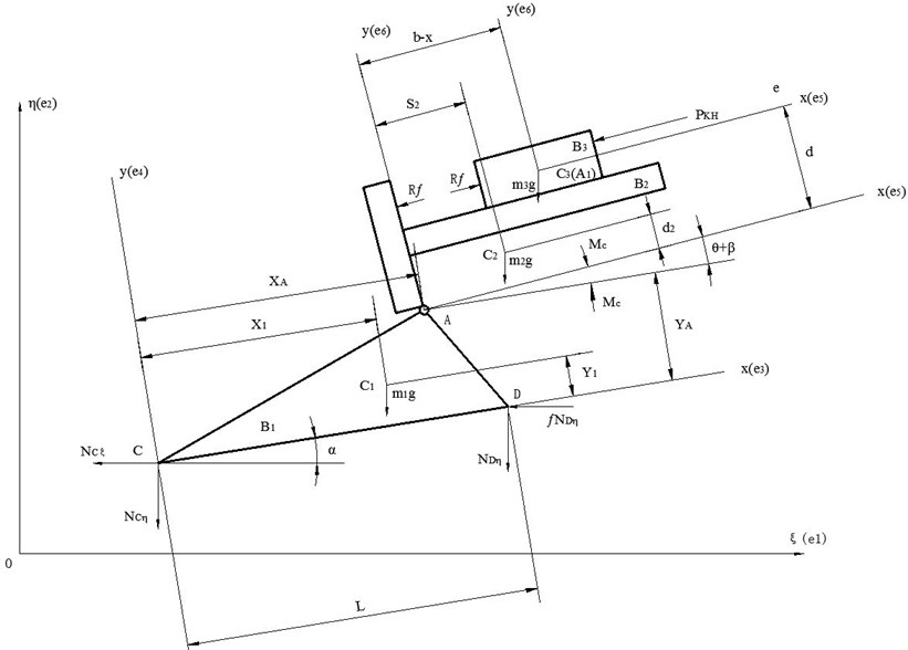
In Fig. 1, $o ξ η$ is chosen as the inertial reference frame; the points $C_{1}$ , $C_{2}$ , $C_{3}$ are center of mass on the rigid body $B_{1}$ , $B_{2}$ , $B_{3}$ ; the points $C$ , $A$ , $A_{1}$ are the base points; the coordinate system $C X Y$ , $A X Y$ , $A_{1} X Y$ is built on these base points; the unit base vector is expressed as $e_{1}$ , $e_{2}$ , $e_{3}$ , $e_{4}$ , $e_{5}$ , $e_{6}$ and $e_{7}$ , where $e_{7}$ is established by right hand rule; $m_{1}$ , $m_{2}$ , $m_{3}$ represents each rigid body’s mass; $m_{1}$ , $m_{2}$ , $m_{3}$ is the rotational inertia relative to $C$ , $A$ , $A_{1}$ ; the force $N_{C ξ}$ and $N_{C η}$ is the constraining force coming from the ground [8-10].

2.2. Dynamic equations

The absolutely velocity and acceleration of each rigid body is illustrated in Eq. (1):

1

\{\begin{array}{l} v_{p 1} = \dot{ξ} e_{1} + \dot{η} e_{2}, \\ a_{p 1} = \ddot{ξ} e_{1} + \ddot{η} e_{2}, \\ v_{p 2}^{} = \dot{ξ} e_{1} + \dot{η} e_{2} - Y_{A} \dot{α} e_{3} + X_{A} \dot{α} e_{4}, \\ a_{p 2}^{} = \ddot{ξ} e_{1} + \ddot{η} e_{2} - (Y_{A} \ddot{α} + X_{A} {\dot{α}}^{2}) e_{3} + (X_{A} \ddot{α} - Y_{A} {\dot{α}}^{2}) e_{4}, \\ v_{p 3}^{} = \dot{ξ} e_{1} + \dot{η} e_{2} - Y_{A} \dot{α} e_{3} + X_{A} \dot{α} e_{4} - d (\dot{α} + \dot{β}) e_{5} - \dot{x} e_{5} + (b - x) (\dot{α} + \dot{β}) e_{6}, \\ a_{p 3}^{} = \{\begin{matrix} \ddot{ξ} e_{1} + \ddot{η} e_{2} - (Y_{A} \ddot{α} + X_{A} {\dot{α}}^{2}) e_{3} + (X_{A} \ddot{α} - Y_{A} {\dot{α}}^{2}) e_{4} \\ - [\ddot{x} + d (\ddot{α} + \ddot{β}) + (b - x) {(\dot{α} + \dot{β})}^{2}] e_{5} \\ + [(b - x) (\ddot{α} + \ddot{β}) - d {(\dot{α} + \dot{β})}^{2} - 2 \dot{x} (\dot{α} + \dot{β})] e_{6} \end{matrix}\}, \\ v_{C 1}^{} = \dot{ξ} e_{1} + \dot{η} e_{2} - Y_{1} \dot{α} e_{3} + X_{1} \dot{α} e_{4}, \\ a_{C 1}^{} = \ddot{ξ} e_{1} + \ddot{η} e_{2} - (Y_{1} \ddot{α} + X_{1} {\dot{α}}^{2}) e_{3} + (X_{1} \ddot{α} - Y_{1} {\dot{α}}^{2}) e_{4}, \\ v_{C 2}^{} = \dot{ξ} e_{1} + \dot{η} e_{2} - Y_{A} \dot{α} e_{3} + X_{A} \dot{α} e_{4} - d_{2} (\dot{α} + \dot{β}) e_{5} + s_{2} (\dot{α} + \dot{β}) e_{6}, \\ a_{C 2}^{} = \{\begin{matrix} \ddot{ξ} e_{1} + \ddot{η} e_{2} - (Y_{A} \ddot{α} + X_{A} {\dot{α}}^{2}) e_{3} + (X_{A} \ddot{α} - Y_{A} {\dot{α}}^{2}) e_{4} \\ - [d_{2} (\ddot{α} + \ddot{β}) + s_{2} {(\dot{α} + \dot{β})}^{2}] e_{5} + [s_{2} (\ddot{α} + \ddot{β}) - d_{2} {(\dot{α} + \dot{β})}^{2}] e_{6} \end{matrix}\}, \\ v_{C 3}^{} = v_{p 3}^{}, \\ a_{C 3}^{} = a_{p 3}^{} . \end{array}

According to Eq. 1, the base vector is expressed in Eq. (2):

2

e_{p}^{v} = [\begin{matrix} \begin{matrix} e_{1} e_{2} \\ e_{1} e_{2} \\ e_{1} e_{2} \end{matrix} & \begin{matrix} 0 \\ X_{A} e_{4} - Y_{A} e_{3} \\ - Y_{A} e_{3} + X_{A} e_{4} - d e_{5} + (b - x) e_{6} \end{matrix} & \begin{matrix} 0 \\ 0 \\ - d e_{5} + (b - x) e_{6} \end{matrix} & \begin{matrix} 0 \\ 0 \\ - e_{5} \end{matrix} \end{matrix}] .

The absolutely angular velocity and angular acceleration of each rigid body is obtained in Eq. (3):

3

\{\begin{array}{l} ω_{1}^{} = \dot{α} e_{7}, \\ {\dot{ω}}_{1}^{} = \ddot{α} e_{7}, \\ ω_{2}^{} = (\dot{α} + \dot{β}) e_{7}, \\ {\dot{ω}}_{2} = (\ddot{α} + \ddot{β}) e_{7}, \\ ω_{3}^{} = (\dot{α} + \dot{β}) e_{7}, \\ {\dot{ω}}_{3} = (\ddot{α} + \ddot{β}) e_{7} . \end{array}

According to Eq. (3), the angular base vector is expressed in Eq. (4):

4

e_{}^{ω} = [\begin{matrix} \begin{matrix} 0 \\ 0 \\ 0 \end{matrix} & \begin{matrix} 0 \\ 0 \\ 0 \end{matrix} & \begin{matrix} e_{7} \\ e_{7} \\ e_{7} \end{matrix} & \begin{matrix} \begin{matrix} 0 \\ e_{7} \\ e_{7} \end{matrix} & \begin{matrix} 0 \\ 0 \\ 0 \end{matrix} \end{matrix} \end{matrix}] .

The principal vector and principal moment of the external force is shown in Eq. (5) and Eq. (7):

5

R^{'} = [\begin{matrix} R_{1} \\ R_{2} \\ R_{3} \end{matrix}],

where:

6

\{\begin{array}{l} R_{1} = \{\begin{array}{l} - (N_{C ξ} c o s ϕ_{1} + N_{C η} s i n ϕ_{1} + f N_{D η} c o s ϕ_{1} + N_{D η} s i n ϕ_{1} + m_{1} g s i n ϕ_{1}) e_{3} \\ + (N_{C ξ} s i n ϕ_{1} - N_{C η} c o s ϕ_{1} + f N_{D η} s i n ϕ_{1} - N_{D η} c o s ϕ_{1} - m_{1} g c o s ϕ_{1}) e_{4} \end{array}\}, \\ R_{2} = - R_{f} e_{5} - m_{2} g s i n ϕ_{2} e_{5} - m_{2} g c o s ϕ_{2} e_{6}, \\ R_{3} = - (P_{K H} - R_{f}) e_{5} - m_{3} g s i n ϕ_{2} e_{5} - m_{3} g c o s ϕ_{2} e_{6} . \end{array}

7

L_{p}^{'} = [\begin{matrix} L_{p 1} \\ L_{p 2} \\ L_{p 3} \end{matrix}],

where:

8

\{\begin{array}{l} L_{p 1} = (M_{C} - N_{D η} L c o s ϕ_{1} + f N_{D η} L s i n ϕ_{1} - m_{1} g X_{1} c o s ϕ_{1} + m_{1} g Y_{1} s i n ϕ_{1}) e_{7}, \\ L_{p 2} = (- M_{C} + R_{f} d_{1} - m_{2} g s_{2} c o s ϕ_{2} + m_{2} g s_{2} s i n ϕ_{2}) e_{7}, \\ L_{p 1} = (P_{K H} e) e_{7} . \end{array}

The principal vector and principal moment of the inertia force is shown in Eq. (9) and Eq. (11):

9

R^{*} = - M a_{C} = - [\begin{matrix} m_{1} & 0 & 0 \\ 0 & m_{2} & 0 \\ 0 & 0 & m_{3} \end{matrix}] [\begin{matrix} a_{C 1} \\ a_{C 2} \\ a_{C 3} \end{matrix}] = [\begin{matrix} - m_{1} a_{C 1} \\ - m_{2} a_{C 2} \\ - m_{3} a_{C 3} \end{matrix}] = [\begin{matrix} R_{1}^{*} \\ R_{2}^{*} \\ R_{3}^{*} \end{matrix}],

where:

10

\{\begin{array}{l} R_{1}^{*} = - m_{1} [\ddot{ξ} e_{1} + \ddot{η} e_{2} - (Y_{1} \ddot{α} + X_{1} {\dot{α}}^{2}) e_{3} + (X_{1} \ddot{α} - Y_{1} {\dot{α}}^{2}) e_{4}], \\ R_{2}^{*} = - m_{2} \{\begin{matrix} \ddot{ξ} e_{1} + \ddot{η} e_{2} - (Y_{A} \ddot{α} + X_{A} {\dot{α}}^{2}) e_{3} + (X_{A} \ddot{α} - Y_{A} {\dot{α}}^{2}) e_{4} \\ - [d_{2} (\ddot{α} + \ddot{β}) + s_{2} {(\dot{α} + \dot{β})}^{2}] e_{5} + [s_{2} (\ddot{α} + \ddot{β}) - d_{2} {(\dot{α} + \dot{β})}^{2}] e_{6} \end{matrix}\}, \\ R_{3}^{*} = - m_{3} \{\begin{matrix} \ddot{ξ} e_{1} + \ddot{η} e_{2} - (Y_{A} \ddot{α} + X_{A} {\dot{α}}^{2}) e_{3} + (X_{A} \ddot{α} - Y_{A} {\dot{α}}^{2}) e_{4} \\ - [\ddot{x} + d (\ddot{α} + \ddot{β}) + (b - x) {(\dot{α} + \dot{β})}^{2}] e_{5} \\ + [(b - x) (\ddot{α} + \ddot{β}) - d {(\dot{α} + \dot{β})}^{2} - 2 \dot{x} (\dot{α} + \dot{β})] e_{6} \end{matrix}\} . \end{array}

11

L_{p}^{*} = - ρ_{C} \times M a_{p} - {\dot{G}}_{p} = - [\begin{matrix} ρ_{C 1} & 0 & 0 \\ 0 & ρ_{C 2} & 0 \\ 0 & 0 & ρ_{C 3} \end{matrix}] \times [\begin{matrix} m_{1} & 0 & 0 \\ 0 & m_{2} & 0 \\ 0 & 0 & m_{3} \end{matrix}] [\begin{matrix} a_{p 1} \\ a_{p 2} \\ a_{p 3} \end{matrix}] - [\begin{matrix} {\dot{G}}_{p 1} \\ {\dot{G}}_{p 2} \\ {\dot{G}}_{p 3} \end{matrix}] = [\begin{matrix} ρ_{C 1} \times (- m_{1} a_{p 1}) - {\dot{G}}_{p 1} \\ ρ_{C 2} \times (- m_{2} a_{p 2}) - {\dot{G}}_{p 2} \\ ρ_{C 3} \times (- m_{3} a_{p 3}) - {\dot{G}}_{p 3} \end{matrix}] = - [\begin{matrix} - ρ_{C 1} \times (- m_{1} a_{p 1}) + {\dot{G}}_{p 1} \\ - ρ_{C 2} \times (- m_{2} a_{p 2}) + {\dot{G}}_{p 2} \\ - ρ_{C 3} \times (- m_{3} a_{p 3}) + {\dot{G}}_{p 3} \end{matrix}] = [\begin{matrix} L_{p 1}^{*} \\ L_{p 2}^{*} \\ L_{p 3}^{*} \end{matrix}],

where:

12

\{\begin{array}{l} L_{p 1}^{*} = \{m_{1} (X_{1} s i n ϕ_{1} + Y_{1} c o s ϕ_{1}) \ddot{ξ} - m_{1} (X_{1} c o s ϕ_{1} - Y_{1} s i n ϕ_{1}) \ddot{η} - J_{1} \ddot{α}\} e_{7}, \\ L_{p 2}^{*} = \{\begin{matrix} m_{2} (s_{2} s i n ϕ_{2} + d_{2} c o s ϕ_{2}) \ddot{ξ} - m_{2} (s_{2} c o s ϕ_{2} - d_{2} s i n ϕ_{2}) \ddot{η} \\ - [J_{2} + m_{2} (s_{2} X_{A} + d_{2} Y_{A}) c o s (ϕ_{2} - ϕ_{1}) + m_{2} (s_{2} Y_{A} - d_{2} X_{A}) \times s i n (ϕ_{2} - ϕ_{1})] \ddot{α} \\ - J_{2} \ddot{β} - m_{2} [(s_{2} X_{A} + d_{2} Y_{A}) s i n (ϕ_{2} - ϕ_{1}) - (s_{2} Y_{A} - d_{2} X_{A}) c o s (ϕ_{2} - ϕ_{1}) {\dot{α}}^{2}] \end{matrix}\} e_{7}, \\ L_{p 3}^{*} = - \{J_{3 C} \ddot{α} + J_{3 C} \ddot{β}\} e_{7} . \end{array}

The generalized force and the generalized moment of force in the whole dynamic model can be expressed in Eq. (13) and Eq. (14):

13

{(e_{p}^{v})}^{T} \cdot R^{'} = [\begin{matrix} \begin{matrix} \begin{matrix} e_{1} \\ e_{2} \end{matrix} \\ 0 \\ \begin{matrix} 0 \\ 0 \end{matrix} \end{matrix} & \begin{matrix} \begin{matrix} e_{1} \\ e_{2} \end{matrix} \\ X_{A} e_{4} - Y_{A} e_{3} \\ \begin{matrix} 0 \\ 0 \end{matrix} \end{matrix} & \begin{matrix} \begin{matrix} e_{1} \\ e_{2} \end{matrix} \\ - Y_{A} e_{3} + X_{A} e_{4} - d e_{5} + (b - x) e_{6} \\ - d e_{5} + (b - x) e_{6} \\ - e_{5} \end{matrix} \end{matrix}] \cdot [\begin{matrix} R_{1} \\ R_{2} \\ R_{3} \end{matrix}] = [\begin{matrix} e_{1} \cdot (R_{1} + R_{2} + R_{3}) \\ e_{2} \cdot (R_{1} + R_{2} + R_{3}) \\ (X_{A} e_{4} - Y_{A} e_{3}) \cdot R_{2} + [- Y_{A} e_{3} + X_{A} e_{4} - d e_{5} + (b - x) e_{6}] \cdot R_{3} \\ \begin{matrix} [- d e_{5} + (b - x) e_{6}] \cdot R_{3} \\ - e_{5} \cdot R_{3} \end{matrix} \end{matrix}],

14

{(e^{ω})}^{T} \cdot L_{p}^{'} = [\begin{matrix} \begin{matrix} \begin{matrix} 0 \\ 0 \end{matrix} \\ e_{7} \\ \begin{matrix} 0 \\ 0 \end{matrix} \end{matrix} & \begin{matrix} \begin{matrix} 0 \\ 0 \end{matrix} \\ e_{7} \\ \begin{matrix} e_{7} \\ 0 \end{matrix} \end{matrix} & \begin{matrix} \begin{matrix} 0 \\ 0 \end{matrix} \\ e_{7} \\ e_{7} \\ 0 \end{matrix} \end{matrix}] \cdot [\begin{matrix} L_{p 1} \\ L_{p 2} \\ L_{p 3} \end{matrix}] = [\begin{matrix} 0 \\ 0 \\ e_{7} \cdot (L_{p 1} + L_{p 2} + L_{p 3}) \\ \begin{matrix} e_{7} \cdot (L_{p 2} + L_{p 3}) \\ 0 \end{matrix} \end{matrix}] .

The generalized inertia force and the generalized inertia moment of force is obtained in a similar way.

Then, by substituting Eq. (1)-(14) into Eq. (15)-(16), the generalized force and the generalized inertia force is established in Eq. (17)-(27):

15

Q = e^{T} \cdot [\begin{matrix} R^{'} \\ L_{p}^{'} \end{matrix}] = {(e_{p}^{v})}^{T} \cdot R^{'} + {(e_{}^{ω})}^{T} \cdot L_{p}^{'},

16

Q^{*} = e^{T} \cdot [\begin{matrix} - M a_{c} \\ - ρ_{c} \times M a_{c} - {\dot{G}}_{p} \end{matrix}] = {(e_{p}^{v})}^{T} \cdot (- M a_{c}) - {(e_{}^{ω})}^{T} \cdot (- ρ_{c} \times M a_{c} - {\dot{G}}_{p}) = {(e_{p}^{v})}^{T} \cdot R^{*} + {(e_{}^{ω})}^{T} \cdot L_{p}^{*},

17

\{\begin{array}{l} Q_{1} = - P_{K H} c o s ϕ_{2} - N_{C ξ} - f N_{D η}, \\ \begin{array}{l} Q_{2} = - P_{K H} s i n ϕ_{2} - (m_{1} + m_{2} + m_{3}) g - N_{C ξ} - N_{D η}, \\ \begin{array}{l} Q_{3} = \{\begin{matrix} P_{K H} [e + d - X_{A} s i n (ϕ_{2} - ϕ_{1}) + Y_{A} c o s (ϕ_{2} - ϕ_{1})] - m_{1} g (X_{1} c o s ϕ_{1} - Y_{1} s i n ϕ_{1}) \\ - (m_{2} + m_{3}) g (X_{A} c o s ϕ_{1} - Y_{A} s i n ϕ_{1}) - m_{2} g (s_{2} c o s ϕ_{2} - d_{2} s i n ϕ_{2}) \\ - m_{3} g [(b - x) c o s ϕ_{2} - d s i n ϕ_{1}] - N_{D η} L c o s ϕ_{1} + f N_{D η} L s i n ϕ \end{matrix}\}, \\ Q_{4} = P_{K H} (e + d) - m_{2} g (s_{2} c o s ϕ_{2} - d_{2} s i n ϕ_{2}) - m_{3} g [(b - x) c o s ϕ_{2} - d s i n ϕ_{1}] - M_{C}, \\ Q_{5} = P_{K H} - R_{f} + m_{3} g s i n ϕ_{2}, \end{array} \end{array} \end{array}

18

Q_{1}^{*} = - (m_{1} + m_{2} + m_{3}) \ddot{ξ} + (m_{1} X_{1} + m_{2} X_{A} + m_{3} X_{A}) s i n ϕ_{1} + (m_{1} Y_{1} + m_{2} Y_{A} + m_{3} Y_{A}) c o s ϕ_{1} + [m_{2} s_{2} + m_{3} (b - x)] s i n ϕ_{2} + (m_{2} d_{2} + m_{3} d_{2}) c o s ϕ_{2}} \ddot{α} + \{[m_{2} s_{2} + m_{3} (b - x)] s i n ϕ_{2} + (m_{2} d_{2} + m_{3} d_{2}) c o s ϕ_{2}\} \ddot{β} + m_{3} c o s ϕ_{2} \ddot{x} + f_{1} = a_{22} \ddot{ξ} + a_{13} \ddot{α} + a_{14} \ddot{β} + a_{15} \ddot{x} + f_{1},

where:

19

f_{1}^{} = \{(m_{1} X_{1} + m_{2} X_{A} + m_{3} X_{A}) c o s ϕ_{1} - (m_{1} Y_{1} + m_{2} Y_{A} + m_{3} Y_{A}) s i n ϕ_{1} + [m_{2} s_{2} + m_{3} (b - x)] c o s ϕ_{2} - (m_{2} d_{2} + m_{3} d) s i n ϕ_{2}\} {\dot{α}}^{2} + \{[m_{2} s_{2} + m_{3} (b - x)] c o s ϕ_{2} - (m_{2} d_{2} + m_{3} d) s i n ϕ_{2}\} ({\dot{β}}^{2} + 2 \dot{α} \dot{β}) - 2 m_{3} \dot{x} (\dot{α} + \dot{β}) s i n ϕ_{2},

20

Q_{2}^{*} = - (m_{1} + m_{2} + m_{3}) \ddot{η} - \{(m_{1} X_{1} + m_{2} X_{A} + m_{3} X_{A}) c o s ϕ_{1} - (m_{1} Y_{1} + m_{2} Y_{A} + m_{3} Y_{A}) s i n ϕ_{1} + [m_{2} s_{2} + m_{3} (b - x)] c o s ϕ_{2} - (m_{2} d_{2} + m_{3} d) s i n ϕ_{2}\} \ddot{α} - \{[m_{2} s_{2} + m_{3} (b - x)] c o s ϕ_{2} - (m_{2} d_{2} + m_{3} d) s i n ϕ_{2}\} \ddot{β} + m_{3} s i n ϕ_{2} \ddot{x} + f_{2} = a_{22} \ddot{η} + a_{23} \ddot{α} + a_{24} \ddot{β} + a_{25} \ddot{x} + f,

where:

21

f_{2}^{} = \{(m_{1} X_{1} + m_{2} X_{A} + m_{3} X_{A}) s i n ϕ_{1} - (m_{1} Y_{1} + m_{2} Y_{A} + m_{3} Y_{A}) c o s ϕ_{1} + [m_{2} s_{2} + m_{3} (b - x)] s i n ϕ_{2} - (m_{2} d_{2} + m_{3} d) c o s ϕ_{2}\} {\dot{α}}^{2} + \{[m_{2} s_{2} + m_{3} (b - x)] s i n ϕ_{2} - (m_{2} d_{2} + m_{3} d) c o s ϕ_{2}\} ({\dot{β}}^{2} + 2 \dot{α} \dot{β}) - 2 m_{3} \dot{x} (\dot{α} + \dot{β}) c o s ϕ_{2},

22

Q_{3}^{*} = \{(m_{1} X_{1} + m_{2} X_{A} + m_{3} X_{A}) s i n ϕ_{1} + (m_{1} Y_{1} + m_{2} Y_{A} + m_{3} Y_{A}) c o s ϕ_{1} + [m_{2} s_{2} + m_{3} (b - x)] s i n ϕ_{2} + (m_{2} d_{2} + m_{3} d) c o s ϕ_{2}\} \ddot{ξ} - \{(m_{1} X_{1} + m_{2} X_{A} + m_{3} X_{A}) c o s ϕ_{1} - (m_{1} Y_{1} + m_{2} Y_{A} + m_{3} Y_{A}) s i n ϕ_{1} + [m_{2} s_{2} + m_{3} (b - x)] c o s ϕ_{2} - (m_{2} d_{2} + m_{3} d) s i n ϕ_{2}\} \ddot{η} - \{J_{1} + J_{2} + J_{3 C} + (m_{2} + m_{3}) (X_{A}^{2} + Y_{A}^{2}) + m_{3} [{(b - x)}^{2} + d^{2}] + 2 [m_{2} s_{2} + m_{3} (b - x)] [X_{A} \cos (ϕ_{2} - ϕ_{1}) + Y_{A} \sin (ϕ_{2} - ϕ_{1})] - 2 (m_{2} d_{2} + m_{3} d) [X_{A} \sin (ϕ_{2} - ϕ_{1}) - Y_{A} \cos (ϕ_{2} - ϕ_{1})]\} \ddot{α} - \{J_{2} + J_{3 C} + m_{3} [{(b - x)}^{2} + d^{2}] + [m_{2} s_{2} + m_{3} (b - x)] \times [X_{A} \cos (ϕ_{2} - ϕ_{1}) + Y_{A} \sin (ϕ_{2} - ϕ_{1})] - (m_{2} d_{2} + m_{3} d) \times [X_{A} \sin (ϕ_{2} - ϕ_{1}) - Y_{A} \cos (ϕ_{2} - ϕ_{1})]\} \ddot{β} + \{m_{3} [X_{A} \sin (ϕ_{2} - ϕ_{1}) - Y_{A} \cos (ϕ_{2} - ϕ_{1})] - m_{3} d\} \ddot{x} + f_{3} = a_{31} \ddot{ξ} + a_{32} \ddot{η} + a_{33} \ddot{α} + a_{34} \ddot{β} + a_{35} \ddot{x} + f,

where:

23

f_{3}^{} = \{[m_{2} s_{2} + m_{3} (b - x)] [X_{A} s i n (ϕ_{2} - ϕ_{1}) - Y_{A} c o s (ϕ_{2} - ϕ_{1})] + (m_{2} d_{2} + m_{3} d) [X_{A} c o s (ϕ_{2} - ϕ_{1}) + Y_{A} s i n (ϕ_{2} - ϕ_{1})]\} ({\dot{β}}^{2} + 2 \dot{α} \dot{β}) + 2 m_{3} [X_{A} c o s (ϕ_{2} - ϕ_{1}) + Y_{A} s i n (ϕ_{2} - ϕ_{1}) + (b - x)] \dot{x} (\dot{α} + \dot{β}),

24

Q_{4}^{*} = \{[m_{2} s_{2} + m_{3} (b - x)] s i n ϕ_{2} + (m_{2} d_{2} + m_{3} d) c o s ϕ_{2}\} \ddot{ξ} - \{[m_{2} s_{2} + m_{3} (b - x)] c o s ϕ_{2} - (m_{2} d_{2} + m_{3} d) s i n ϕ_{2}\} \ddot{η} - \{J_{2} + J_{3 C} + m_{3} [{(b - x)}^{2} + d^{2}] + [m_{2} s_{2} + m_{3} (b - x)] \times [X_{A} c o s (ϕ_{2} - ϕ_{1}) + Y_{A} s i n (ϕ_{2} - ϕ_{1})] - (m_{2} d_{2} + m_{3} d) \times [X_{A} s i n (ϕ_{2} - ϕ_{1}) - Y_{A} c o s (ϕ_{2} - ϕ_{1})]\} \ddot{α} - \{J_{2} + J_{3 C} + m_{3} [{(b - x)}^{2} + d^{2}]\} \ddot{β} + m_{3} d \ddot{x} + f_{4} = a_{41} \ddot{ξ} + a_{42} \ddot{η} + a_{43} \ddot{α} + a_{44} \ddot{β} + a_{45} \ddot{x} + f,

where:

25

f_{4}^{} = - \{[m_{2} s_{2} + m_{3} (b - x)] [X_{A} s i n (ϕ_{2} - ϕ_{1}) - Y_{A} c o s (ϕ_{2} - ϕ_{1})] + (m_{2} d_{2} + m_{3} d) [X_{A} c o s (ϕ_{2} - ϕ_{1}) + Y_{A} s i n (ϕ_{2} - ϕ_{1})]\} {\dot{α}}^{2} + 2 m_{3} (b - x) \dot{x} (\dot{α} + \dot{β}),

26

Q_{5}^{*} = m_{3} c o s ϕ_{2} \ddot{ξ} + m_{3} s i n ϕ_{2} \ddot{η} + m_{3} [X_{A} s i n (ϕ_{2} - ϕ_{1}) - Y_{A} c o s (ϕ_{2} - ϕ_{1})] \ddot{α} - m_{3} d \ddot{β} - m_{3} \ddot{x} + f = a_{51} \ddot{ξ} + a_{52} \ddot{η} + a_{53} \ddot{α} + a_{54} \ddot{β} + a_{55} \ddot{x} + f_{5},

where:

27

f_{5}^{} = - m_{3} [X_{A} c o s (ϕ_{2} - ϕ_{1}) + Y_{A} s i n (ϕ_{2} - ϕ_{1})] {\dot{α}}^{2} - m_{3} (b - x) (\dot{α} + \dot{β}) .

Finally, the whole mechanism dynamic equations are established as Eq. (28):

28

A \ddot{q} = F,

where:

29

A = [\begin{matrix} a_{11} & a_{12} & \dots & a_{15} \\ a_{21} & a_{22} & \dots & a_{25} \\ \dots & \dots & \dots & \dots \\ a_{51} & a_{52} & \dots & a_{55} \end{matrix}],

30

q = {[\begin{matrix} \begin{matrix} ξ & η \end{matrix} & α & β & x \end{matrix}]}^{T},

31

F = {[\begin{matrix} \begin{matrix} - (Q_{1} + f_{1}) & - (Q_{2} + f_{2}) \end{matrix} & - (Q_{3} + f_{3}) & - (Q_{4} + f_{4}) & - (Q_{5} + f_{5}) \end{matrix}]}^{T} .

3. Field experiment

In order to identify the time-varying system parameters, like time-varying mass, a field experiment is designed and conducted.

3.1. Experimental equipment

Experiment Equipment mainly consists of two parts, the data collection system and the high-speed photography system.

The data collection system consists of Brüel&Kjær acceleration sensor, Qiwei angular acceleration sensor, Lianneng pressure sensor, Kistler charge amplifier, Dewetron data collector, Dewetron software and so on.

The high-speed photography system consists of an IDT Y3-S2 high-speed camera, a high-light LED light, a nikkor 50 mm/1.2D camera lens, a nikkor 400 mm/2.8D camera lens, ProAnalyst dynamic target capture software and some other ancillary equipment.

3.2. Experiment results

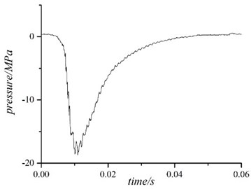
The angular velocity of the recoiling part is shown in Fig. 2 and the active force of the mechanism system is shown in Fig. 3.

Fig. 2The angular velocity of the recoiling part

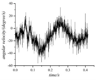
Fig. 3The active force of the mechanism system

4. Numerical calculation

4.1. Identification method

The model can be expressed in Eq. (32) [11-13]:

32

A (z^{- 1}) y (k) = B (z^{- 1}) y (k - d) + ξ (k),

where $ξ (k)$ is white noise, and the structure parameters $m$ , $n$ , $d$ are known. And:

33

\{\begin{array}{l} A (z^{- 1}) = 1 + a_{1} z^{- 1} + a_{2} z^{- 2} + \cdot \cdot \cdot + a_{m} z^{- m}, \\ B (z^{- 1}) = b_{0} + a_{1} z^{- 1} + a_{2} z^{- 2} + \cdot \cdot \cdot + a_{n} z^{- n} . \end{array}

The target of identification is to establish $m + n + 1$ parameters according to the measurable input and output. The model can be described in least square method and is expressed in Eq. (34):

34

y (k) = - a_{1} y (k - 1) - \cdot \cdot \cdot - a_{n_{a}} y (k - n_{a}) + b_{0} u (k - d)

+ \cdot \cdot \cdot + b_{n_{b}} u (k - d - n_{b}) + ξ (k) = φ^{T} (k) θ + ξ (k),

where $φ (k)$ is the data vector, $θ$ is the parameter need to be identified. And:

35

\{\begin{array}{l} φ (k) = {[- y (k - 1), \cdot \cdot \cdot, - y (k - n_{a}), u (k - d), \cdot \cdot \cdot, u (k - d - n_{b})]}^{T} \in R^{(n_{a} + n_{b} + 1) \times 1}, \\ θ = {[a_{1}, \cdot \cdot \cdot, a_{n_{a}}, b_{0}, \cdot \cdot \cdot, b_{n_{b}}]}^{T} \in R^{(n_{a} + n_{b} + 1) \times 1} . \end{array}

So, the identification equation of the rigid body mechanism model can be expressed in Eq. (36):

36

m_{3} {\ddot{q}}^{'} = F^{'} .

4.2. Identification results

The time-varying identified mass of the recoiling part is illustrated in Fig. 4.

Fig. 4The time-varying identified mass of the recoiling part

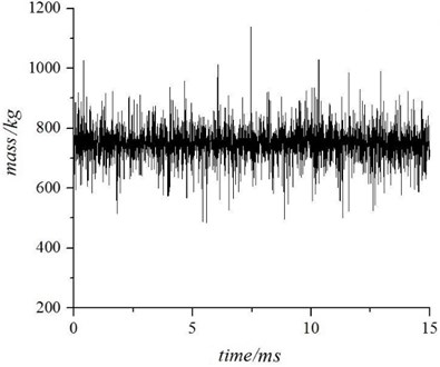
The angular velocity data contains the stress wave noise, as a result that the identified mass of the recoiling part consists of calculative deviation. Although, this time-varying identified mass can reflect the calculative consequence ignoring physical significance.

A relative percentage error (RPE) is defined to compare the result of the identification which is expressed in Eq. (37):

37

R P E = \frac{Σ | m_{t r u e} - m_{i d e n t i f y} |}{Σ | m_{t r u e} |} \times 100 % .

In Fig. 4, the identified mass of the recoiling part is about 740 kg. After comparing with the “real” mass which was consulted in mechanism specification book, the RPE is finally established at about 5.4 %.

5. Conclusions

In this paper, the multi-rigid-body theory and the limited memory least square method is applied to identify the time-varying mass of the recoiling part.

The mass of the recoiling part has physical significance so that the result of identification can be compared to the static measurement which is consulted in mechanism specification book. Limited memory least square method can overcome “data saturation” phenomenon effectively and it can be applied to time-varying identification in this situation. The result reflects that limited memory least square method and the process of establishing the mechanism dynamic equations are accurate in identifying the time-varying mass. At the same time, a new kind of identification method is provided to make the parameters more intuitive and can be applied in identifying dynamic loads which is difficult to measure.

At the present stage, the dynamic model is described as rigid body model. In the future, this model would be instead of flexible multi-body model to make the equations more accurately. And more parameters would be identified such as the mass and the stiffness of the structure, the active force from the propellant powder, the inertia force of the mechanism.

References

Chen Q., Yang G., Zhu Z. Gun dynamics analysis based on wavelet. Journal of Gun Launch and Control, Vol. 2, 2009, p. 37-40.

Search CrossRef
Rui X., Dang S., Zhang Q., Lu Y. Multi-body transfer matrix method on artillery. Dynamics Mechanics in Engineering, Vol. 17, 1995, p. 42-43.

Search CrossRef
Jing D., Liu X. Identifying physical parameters of joint moving state robots. Journal of Beijing University of Posts and Telecommunications, Vol. 31, 2008, p. 52-55.

Search CrossRef
Jing D., Liu X. On-line identification of time-varying physical parameters of robot joint based on harmonic propagation. Journal of Vibration Engineering, Vol. 45, 2009, p. 296-301.

Search CrossRef
Zhuang W., Liu X. Joint parameters identification of robot based on traveling wave approach and neural network. Journal of Vibration Engineering, Vol. 23, 2010, p. 173-178.

Search CrossRef
Chen X., Chen C. Parameter identification of time-varying systems based on the least-squares modified algorithm. Journal of Fuzhou University, Natural Science, Vol. 33, Issue 2, 2007, p. 163-166.

Search CrossRef
Fedaravičius A., Jonevičius V., Survila A., Pincevičius A. Dynamics study of the carrier HMMWV M1151. Journal of Vibroengineering, Vol. 15, Issue 3, 2013, p. 1619-1626.

Search CrossRef
Theoretical Mechanics Teaching and Research Section of Harbin Institute of Technology, Theoretical Mechanics. Higher Education Press, Beijing, 2002.

Search CrossRef
Kang X., Ma M., Wei X. Modeling theory of gun system. National Defense Industry Press, Beijing, 2003.

Search CrossRef
Zhang Y. Mechanical Vibration. Tsinghua University Press, Beijing, 2007.

Search CrossRef
Chen Q., Wang M., Yan H., Ye H., Yang G. An adaptive method for inertia force identification in cantilever under moving mass. Journal of Vibroengineering, Vol. 14, Issue 3, 2012, p. 1052-1058.

Search CrossRef
Chen Q., Yan H., Wang M., Ye H. Inertia force identification of cantilever under moving-mass by inverse method. Telkomnika, Vol. 10, Issue 8, 2012, p. 2108-2116.

Search CrossRef
Xu R., Chen Q., Yang G. Identification of robot arm’s joints’ time-varying stiffness under loads. Telkomnika, Vol. 10, Issue 8, 2012, p. 2081-2087.

Search CrossRef

About this article

Received

01 November 2013

Accepted

10 November 2013

Published

15 February 2014

Keywords

multi-body dynamics

mass

identification

limited memory least square method

Acknowledgements

This work was supported in part by the Major State Basic Research Development Program of Republic of China (No. 613116).

This is an open access article distributed under the Creative Commons Attribution License, which permits unrestricted use, distribution, and reproduction in any medium, provided the original work is properly cited.