Dynamics analysis of electric shoegear and conductor rail system

1. Introduction

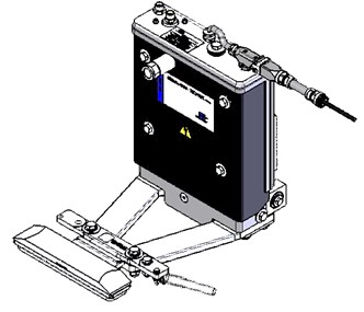
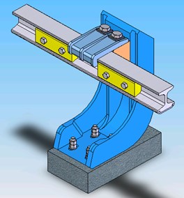
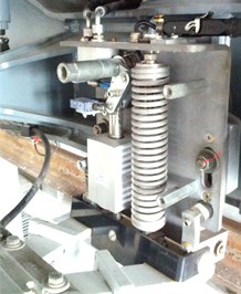
Electric shoegear and conductor rail system as shown in Fig. 1, is one of the most traditional traction power supply methods for electric trains. Since 1890 when the world first conductor rail railway opened in London, electric shoegear and conductor rail system has been widely used in urban rail transportation, and its highest speed has reached 174 km/h [1]. With increasing urban construction scale in China, the original train speed limit, 80 km/h, obviously cannot meet requirements of long interval. Therefore it is imperativeto develop a system that allows operation speed up to 120 km/h or even 160 km/h. As known, the higher speed makes more intensive vibration in electric shoegear and conductor rail system. The service life of the system may be shorten due to the wear between the shoegear and the rail, and the maintenance costs may increase. If the shoegear is separated from the rail, serious problems such as derailment may be caused by the unstable collection of electric energy. In order to develop an electric shoegear and conductor rail system for a higher speed, it is need to research its dynamic characteristic.

There are many researches in dynamics of electric shoegear and conductor rail system: T. Teng [2] built a multi-rigid-body model of electric shoegear and conductor rail, and found the vibration law of the system by changing parameters such as track smoothness and electric shoegear. P. F. Weston [3] obtained the relationship between the displacement of electric shoegear and the contact force. However, T. Teng [2] and P. F. Weston [3] both did not give the dynamic equations. Electric shoegear is mobile equipment while conductor rail is fixed facility. The shoegear slides on conductor rail at working which can be equivalent to a moving load working on a beam. Considering this mechanism, there are many researches: J. Zhao [4] obtained the response of beam vibration under a moving load, however inertia was not considered; Q. Chen [5] involved inertia of moving mass as an additional dynamic stiffness matrix and solved the response of a beam by Wittrick-Williams method; V. Gasic [6] and B. Dyniewicz [7] used finite element method (FEM) to solve contact force by involving a control equation into dynamic equations through Newmark integration; G. Visweswara [8] solved moving mass beam equations by using perturbation modal coordinates while M. Foda [9] used dynamic Green’s function and others [10-12] used mode superposition method to solve the same problem. However in these researches, the moving load is treated as a particle and cannot be used in electric shoegear and conductor rail system, because electric shoegear is a rotation driver containing stiffness and damping. Therefore it is need to establish an appropriate model for electric shoegear and conductor rail system.

Fig. 1. Electric shoegear and conductor rail system

a)

b)

In this paper, the author first simplified electric shoegear and conductor rail system as a cantilever with rotating mechanism attaching to a simply-supported Euler-Bernoulli beam. Then assuming that there is no separation between them, through mechanics analysis, the author obtained dynamics equations of electric shoegear and conductor rail system, which is the analytical model. Based on the analytical model, numerical solution can be got by using numerical integration method. Considering it is hard to get the solution of analytical model in practical, a numerical model of the system was built by FEM, and parameters were measured in vibration tests. Finally, the author explored the vibration rules of electric shoegear and conductor rail system by substituting operation parameters.

2. Dynamic equations of electric shoegear and conductor rail system

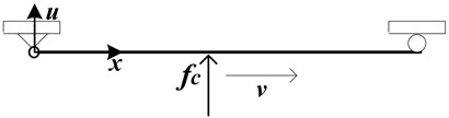
Conductor rail is similar to normal rail in geometric but with a smaller section area. Comparing to length of the rail, its section area can be ignored and then the rail would be equivalent to a Bernoulli-Euler beam, as shown in Fig. 2. Its dynamic equation is as follow:

where, $u(x,t)$ is vertical displacement of the beam, $0\le x\le L$, $0\le t\le L/v$, $\rho A$ is mass of conductor rail in unit length, $EI$ is Young’s modulus of the conductor rail, $x$ is displacement along the beam, $L$ is length of a cross beam, $v$ is moving speed of contact force, $\delta \left(x-vt\right)$ is Dirac function. When the force moves to $x=v\times t$, $\delta$ equals to 1.

Fig. 2Dynamics model of conductor rail

The boundary conditions are ${\left.u\left(x,t\right)\right|}_{x=0,L}=0\text{,}$${\left.\frac{{\partial }^{2}u\left(x,t\right)}{\partial x^2}\right|}_{x=0,L}=0$ and the initial conditions are ${\left.u\left(x,t\right)\right|}_{t=0}=0$, ${\left.\frac{\partial u\left(x,t\right)}{\partial t}\right|}_{t=0}=0$.

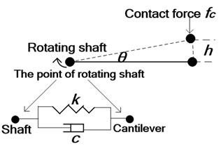
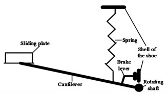
Fig. 3 sketches that ashoegear connects to conductor rail as a cantilever whose torsion is supplied through a rotating shaft. It is assumed that the cantilever is a mass-rod structure: there is a mass at one end of the rod attaching to conductor rail. According to Fig. 4, dynamic equation of electric shoegear is as follow:

where ${\theta }_0$ is initial rotation angle of cantilever of the shoegear, $k$ is rotational stiffness, $c$ is rotational damping, $l$ is length of cantilever, $m$ is equivalent mass of the shoegear, $N$ is initial contact force, $N=k{\theta }_0/l$.

Fig. 3Model of electric shoegear

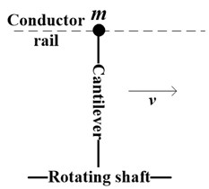
Fig. 4Force analysis of electric shoegear

It is acceptable to assume that the rotation of the electric shoegear is very small, which leads $\theta ={\mathrm{s}\mathrm{i}\mathrm{n}}^{-1}\left(\mu \left(t\right)/l\right)\approx \mu \left(t\right)/l$. Taking it into Eq. (2) and ignoring damping of the electric shoegear, Eq. (2) can be rewrote in:

A simple contact model of electric shoegear and conductor rail system is as shown in Fig. 5, that the contact force caused by a spring makes the shoegear closely contact to the rail. Comparing to the displacement of the electric shoegear, removing to the center of line due to the rotation can be neglected.

Fig. 5Electric shoegear and conductor rail system

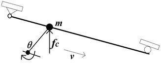
Shoegear slides on the conductor rail so it is acceptable to presume that shoegear and rail always stay together, therefore it can be got:

Make second derivation of Eq. (4), then:

To substitute Eq. (3) and Eq. (5) into Eq. (1), it is got:

Eq. (6) is the dynamic equation of electric shoegear and conductor rail system. It can be seen that it is a 2-DOF system present by a 2-order partial differential equation, including vibration of the beam and an external load.

3. Solution of dynamic equation

In this paper, Lagrange equations are used to solve Eq. (6). Firstly, the total kinetic energy and potential energy of the system can be respectively present as:

Assuming that functions of the displacement of the shoegear and rail is as follow:

Taking Eq. (9) and Eq. (10) into Eq. (7) and Eq. (8), it is got:

Due to the orthogonally of formation:

Substituting in Eq. (11) and Eq. (12), we obtain:

According to the Second Lagrange equation:

Taking Eq. (14) and Eq. (15) into Eq. (16), the equation of system vibration response can be obtained:

Eq. (17) can be expanded and equivalent in $i$th order, which means that ${\xi }_i\left(t\right)$ has infinite DOFs. Since $i=j=$1, 2,…, $n$, it can be arranged in matrix as:

Taking boundary conditions and initial conditions into Eq. (18), using Newmark-β integration method, we obtain values of ${\xi }_i\left(t\right)$ which can be substituted into Eq. (9) and Eq. (10) to get the dynamic response of displacement of the beam and the particle.

Rearranging Eq. (2) and taking it into Eq. (10), the contact force can be present as:

The Newmark integration method is based on the assumption that the acceleration varies linearly between two instants of time. The Newmark’s equations in standard form:

$\mathrm{\Delta }t$ in Eq. (20) and Eq. (21) is the integration time. ‘$\beta$’ and ‘$\gamma$’ arecoefficients which are usually 0.25 and 0.5 respectively so that at such conditions, the solution is unconditional convergence. Details can be found in reference [13].

4. Examples of analytical model

To solve the Eq. (18) is equivalent to get DOFs of coordinate in $n$th modals. Take $n=$3 as an example to illustrate the dynamic response of electric shoegear and conductor rail system.

To bring the parameters in Table 1 in Eq. (18) and set integration time as 1000, we can calculate ${\xi }_1\left(t\right)$, ${\xi }_2\left(t\right)$, ${\xi }_3\left(t\right)$ by using speeds 4.8 m/s, 24 m/s and 48 m/s respectively, and take the results into Eq. (9) and Eq. (10) to get the vibration response of the displacement of shoegear and rail. Then the response curves of contact force can be plotted by substituting displacement of the shoegear into Eq. (19).

When the speed is 48 m/s, it is easy to get three modal coordinates and plot its 1st and 2nd modal coordinates ${\xi }_1\left(t\right)$, ${\xi }_2\left(t\right)$ in Fig. 6. It can be seen that amplitude of 1st modal coordinates is larger thanthe one of 2nd model.

Fig. 6Modal coordinate curves at 48 m/s

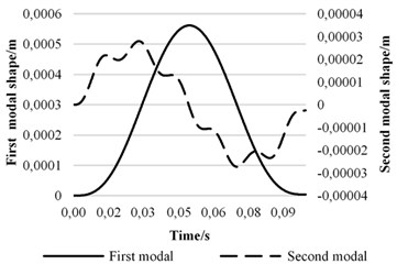
Fig. 7Displacement curves in different positions of beam at 48 m/s

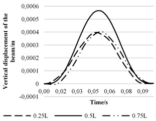
Fig. 7 shows the displacement curves of three different points on the beam when the speed is 48 m/s. As we can see, the maximum vibration occurs at 0.5$L$ that is up to 5.6 mm, and the vibration at 0.75$L$ lags than the one at 0.25$L$. Considering Fig. 6, to displacement response of the beam, 1st modal coordinate contributes most.

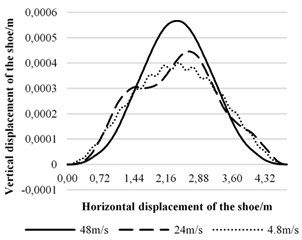
Fig. 8 shows displacement of the middle point of beam at different speeds. Fig. 9 that shows the trajectories of electric shoegear, which can be obtained by substituting modal coordinates into Eq. (10). Comparing Fig. 8 and Fig. 9, it is noticed that the trajectory of electric shoegear is similar to the displacement of the middle point of beam.

Fig. 8Displacement curves in the middle of beam at different speeds

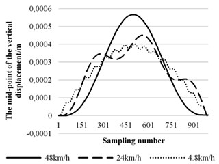
Fig. 9Trajectories of the shoegear at different speeds

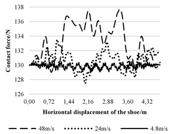
According to Eq. (19), contact force curves can be drawn as shown in Fig. 10. As speed increasing from 4.8 m/s to 48 m/s, standard deviation of contact force increases from 0.29 N to 2.5 N. In other words, fluctuation of contact force becomes violent.

Fig. 10Contact force curves at different speeds

5. Vibration measurement of electric shoegears and its modeling

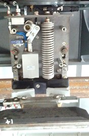
Electric shoegears are mounted on sides of electrified train bogies (as shown in Fig. 11), collecting current from conductor rail and supplying power to electric equipment on board. Electric shoegears are mainly assembled by a prestressed spring, bearings, insulation connectors, a brake lever and a sliding plate and its bracket etc. As shown in Fig. 12, contact force between conductor rail and sliding plate caused by spring and transmitted by bearings, makes current well-collected from the rail to traction units through electric connectors.

In addition, following assumptions are made: taking bracket of sliding plate and insulation connector as one part, as a cantilever; ignoring the height difference cause by spring connectors, that’s to say, the spring is connected to the cantilever directly; taking brake lever used to limit maximum operation height, as a part of cantilever; assuming all connection is linear including linear stiffness and damping.

Fig. 11Internal structure of electric shoegear

a)

b)

Fig. 12 indicates that height of sliding plate affects contact force directly, that at different height contact force provided by spring is different. To change the height, the contact force need to reach a threshold value. Brake lever limits operation height of shoegears so that shoegears can leave the rail when it goes higher.

Fig. 12Transmission principle of electric shoegear

Movement principle of electric shoegears is similar to lever principle: bearing works as a fulcrum while cantilever balances contact force and spring force.

Known from transmission principle of electric shoegears, the key is to calculate three parameters: stiffness of the spring, distance ratio of axis of spring and sliding plate to rotating shaft and the rotating angle of cantilever. In this paper, the three parameters are obtained through a series of tests.

The purpose of vibration tests is to measure key parameters of electric shoegears, which are used to established FEM model of electric shoegears according to the transmission principle.

In tests, the statics (height of sliding plate with different static forces) and the dynamics (displacement-time curve of sliding plate with sudden force change) of electric shoegears are obtained by loading different force on sliding plate.

Fig. 13Arrangement of tests

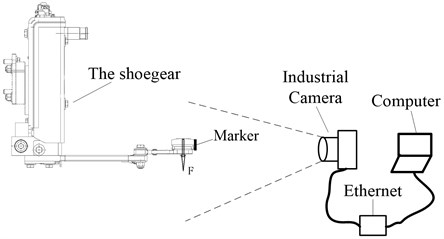
Fig. 14Image captured by industrial camera

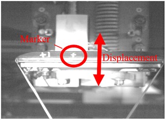
The arrangement of test shows in Fig. 13 that the displacement of sliding shoegear is recorded visually in real time. There is a painted marker on the sliding plate whose vertical displacement is recognized and recorded by an industrial camera directly connecting to a computer via Ethernet. Fig. 14 is an image recorded by the industrial camera where the marker ‘+’ is circled.

Following parameters of electric shoegear can be measured:

1) The distance between rotating shaft and center of sliding plate is 428 mm;

2) The distance between rotating shaft and spring is 65 mm;

3) Total weight of sliding plate including its bracket and insulation plate is 8.914 kg.

Static analysis is to obtain real position of the shoegear when friction is ignored. The position is calculated by taking average of displacement in positive direction and negative direction when load on sliding plate changes. Fig. 15 gives measured values and their mean values under 120 N, 130 N, 135 N and 140 N.

Fig. 15Analytical result of statics

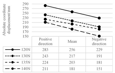
The static parameters measured visually are as follow:

1) The vertical force when sliding plate begins to move is 120 N;

2) The vertical force when sliding plate stays in horizon is 135 N;

3) The distance between maximum operation height of sliding plate and rotating shaft is 53 mm;

4) When taking 130 N load, height of sliding plate decreases 39 mm;

5) When taking 140 N load, height of sliding plate decreases 75 mm.

Set sliding plate stays static with 140 N load. Suddenly removing 10 N load, the sliding plate begins to vibrate, and the motion curve is recorded by the camera and shown in Fig. 16.

Fig. 16Motion curve of sliding plate when loads change from 140 N to 130 N

The first three complete cycles in Fig. 16 respectively are 0.474 s, 0.470 s, 0.472 s and their mean value is 0.472 s so that the natural frequency of electric shoegear can be calculated as 2.1 Hz. If vibration amplitude becomes less than 1 mm, the vibration can be thought to be end, so the transient vibration lasts 2.7 s.

According to movement principle of electric shoegears, FEM model can be built as shown Fig. 17 with following measured parameters (to the beam, the length is 428 mm while the angle is 7.06°; as to the spring unit, the length is 65 mm while the angle is 7.06°) and actual parameters (mass of beam unit is 8.914 kg as measured and its section area is 150 mm×50 mm). To achieve the effect of brake lever, cable unit is connected to one end of cantilever and at the maximum working height, cable becomes tight so cantilever cannot go upward. However, below the maximum working height, the cable is in compression so it can be ignored.

FEM model of electric shoegear consists of a rotating hinge unit and a beam with two real parameters, sliding plate and frame. The beam element of electric shoegear is a 3-dimension unit as shown in Fig. 17, whose nodes’ DOFs are:

The mass and stiffness matrix refers to Reference [15]. Composite beam is in the same form of conductor rail:

As shown in Fig. 4, rotation unit that has 2 DOFs is in the form of Eq. (2). Because of the axial DOF of three-dimension beam unit, the finite element Equation can be got by substituting Eq. (2) into Eq. (23):

where $r$ is adjusted to row of rotating unit’s DOFs.

Fig. 17FEM model of electric shoegear

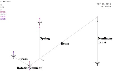
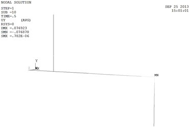
Fig. 18Node displacement of electric shoegear when load is 140 N

The only unknown parameters are stiffness of the spring unit and the rotation friction of the rotation unit, but the spring stiffness can be measured by statics test.

After calculating, setting stiffness of the spring 11300 N/m, static displacement of electric shoegear matches the average measured in the test as shown in Table 2. When the load increases to 140 N, displacement of nodes is present in Fig. 18.

Rotation friction of electric shoegears is superimposed of many dry friction pairs that are unrelated to rotation angle and in opposite direction. Since the friction force is ignored in calculation, here take rotation friction as a viscous damping that is proportional to the rotation angle and in value of 0.5 Nm/rad through calculating.

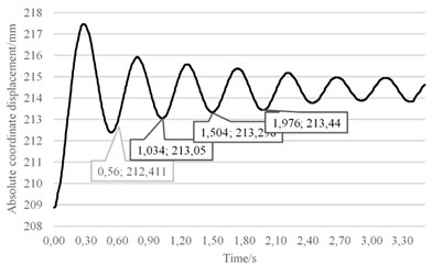
First taking the sliding plate at standstill, then changing load from 140 N to 130 N, sliding plate begins to vibrate and its displacement-time curve is shown in Fig. 19.

Fig. 19Simulated motion curve of sliding plate when loads change from 140 N to 130 N

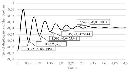
The first three complete cycles in Fig. 19 respectively are 0.45 s, 0.4725 s, 0.45 s and their mean value is 0.4575 s so that the natural frequency of electric shoegear is 2.19 Hz. If vibration amplitude becomes less than 1 mm, the vibration is thought to be end, so the transient vibration lasts 2.54 s.

According to data above, simulation results basically tallies with test value. Comparing Fig. 16 and Fig. 19, amplitude in simulation is much larger than it in tests, for nonlinear friction of electric shoegears is neglected in the simulation model.

6. FEM model of conductor rail

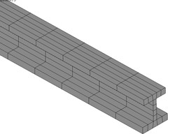
Conductor rail is laid along the track on the ground and used to supply power to electric shoegears. Section of conductor rail is shown in Fig. 20. The rail usually consists of an aluminum alloy base covered by a layer of stainless steel as conductive surface.

Fig. 20Section of conductor rail

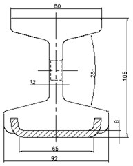
Fig. 21Sketch of arrangement of conductor rail

To build up model of conductor rail, stainless steel part and aluminum part are considered as one calculated by same elasticity modulus, while density equals mass of unit length divide by section area.

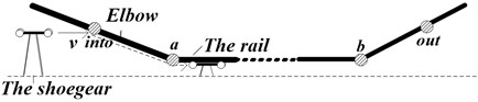
At both ends of conductor rail, there are elbows used to make electric shoegears slide in and out the rail smoothly as shown in Fig. 21. Between point ‘$a$’ and ‘$b$’, the rail is flat.

By using finite element method, continuous conductor rail can be divided into many beam units and fixing base can be seen as a spring as model in Fig. 22.

Analytical calculation is complicated in this condition because spans are different and slope changes at ends. In this paper, the author established FEM models of electric shoegear and conductor rail, then combined them by contact algorithm and finally solved the dynamic matrix by Newmark-$\beta$ numerical integration.

The structure of conductor rail can be treated as many 4-DOFs beam units (see Fig. 22), in which the support point can be adjusted by span length and denoted by a spring. To a random beam unit, 4 DOFs of 2 nodes wherein a beam unit can be present in a local coordinate system:

where, $u\left(t\right)$ is vertical displacement of contact rail, $u^{*}\left(t\right)$ is moment of contact rail, $l$ is length of a beam element, $f\left(t\right)$ is the load of contact rail.

Eq. (25) can be simplified:

Considering Eq. (25) is in its local coordinates, change it into the global coordinates:

where [$T$] (the transformation matrix) reads:

In Eq. (28), $\alpha$ is the angle between local coordinates and global coordinates, whose positive direction is counterclockwise.

In Fig. 22, fixing points were suspended by a spring whose stiffness is $k_1$. So the stiffness matrix of fixing point becomes:

where $n$ is number of suspension points.

Since suspension point is at a node of the beam unit, $k_1$ in Eq. (29) may be in the row of $u_i$ or $u_j$.

Therefore the integral finite element equations can be obtained from Eq. (27):

FEM model of conductor rail (see Fig. 23) matches the dimension in Fig. 20.

Fig. 22Discrete units of conductor rail

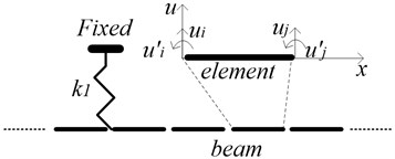
Fig. 23FEM model of conductor rail

7. Contact model of electric shoegear and conductor rail

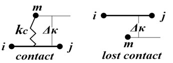
Based on FEM model of electric shoegear and conductor rail, penalty function method is chosen to use to establish contact model of electric shoegear and conductor rail. To assume that there are two contact points on the shoegear, the contact model can be built as shown in Fig. 24, where $m$ is one of contact points and $i$ and $j$ are nodes of rail beam. When $m$ moves to $i-j$ unit, the perpendicular distance $\mathrm{\Delta }\kappa$ from $m$ to $i-j$ should be greater than 0. The plus-minus sign of $m$ shows whether electric shoegear and conductor rail are connected. If $\mathrm{\Delta }\kappa$ is greater than 0, there is contact force in value of:

$\mathrm{\Delta }\kappa$ depends on the perpendicular distance between contact points and upper beam unit of conductor rail. If direction of $w$ is in the same direction of $u$, then:

If $\mathrm{\Delta }\kappa$ is less than 0, contact force is given 0.

Fig. 24Contact model of electric shoegear and conductor rail

8. Transient vibration model example

Parameters of conductor rail can be found in Table 1 and Fig. 20. Set the left end of flat section as the origin of coordinates and sketch of arrangement of conductor rail can be got in Fig. 21. Total length of conductor rail is 23.2 m and support points are at following positions: 0.8 m, 4.4 m, 9.2 m, 14.0 m, 18.8 m, and 22.4 m. The stiffness of the support points is 10000 N/m.

Parameters of electric shoegears can be found in chapter 4. According to EN 50318 [16], the contact stiffness $k_c$ between electric shoegear and conductor rail is given 50000 N/m.

At last, the FEM model can be solved by Newmark-$\beta$ numerical integration to simulate the vibration response. In each time step, contact force should re-calculate according to moving speed and displacement of electric shoegear. That’s to say, contact force is a changing load in every time step.

The contact force of electric shoegear and conductor rail at different speeds can be calculated and plotted in Fig. 25.

As we can see, contact force decreases at first, then re-decreases into a comparatively stable status after amplitude regaining. When electric shoegear goes under rail, they crash and vibrate violently. However as the action goes, acceleration and contact force decrease until the shoegear arrives at turning point. At turning point, contact force increases immediately and then decreases slightly on flat part. During the shoegear leaving, contact force trends to be stable.

Fig. 25Curve of contact force at different speeds

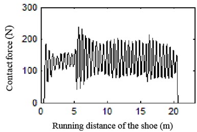
a) 60 km/h

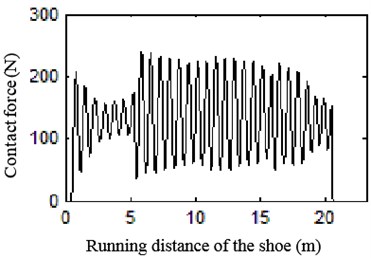
b) 80 km/h

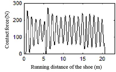
c) 120 km/h

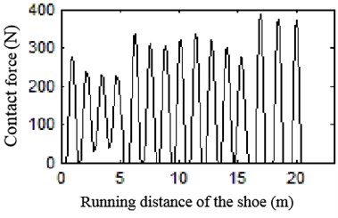
d) 140 km/h

Fig. 26Curve of acceleration of sliding plate at different speeds

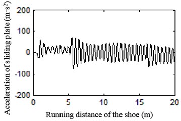
a) 60 km/h

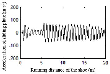
b) 80km/h

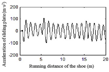
c) 120 km/h

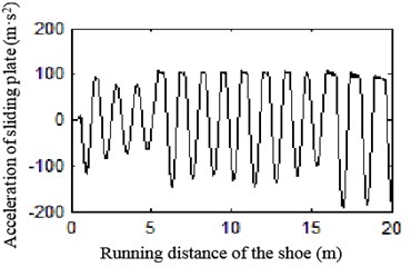
d) 140 km/h

Fig. 26 shows the vertical acceleration of electric shoegear’s sliding plate. As we can see, as the increase of speed, the vibration becomes more violent.

Values of Fig. 25 are counted in Fig. 27, which shows average of contact force is about 134 N and increasing with speed. Standard deviation of contact force increases rapidly from 120 km/h and reaches 117 N at 140 km/h that indicates the contact between electric shoegear and conductor rail is in harsh condition and very likely to be separated.

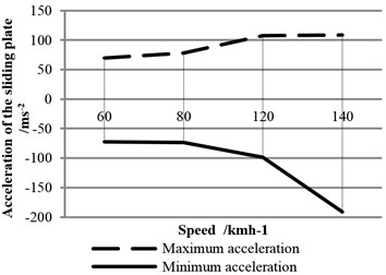
Numeral statistics of Fig. 26 is plotted in Fig. 28, which shows vibration acceleration of sliding plate ascends with growth of speed. When speed is 140 km/h, the acceleration is approaching 200 m/s², which is almost twice as much as the value at 120 km/h.

Fig. 27Statistics of contact force at different speeds

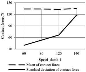
Fig. 28Statistics of acceleration of the sliding plate at different speeds

As speed goes higher, volatility of contact force increases. But it is satisfied if electric shoegear does not leave conductor rail (contact force decreases to 0). When shoegears are offline, electric trains cannot collect current from the rail. Fig. 29 shows offline numbers at different speeds: 1 time offline occurs at 120 km/h while the number roars to 9 when speed is 140 km/h. according to offline numbers, it is suggested that the maximum operation speed should be 120 km/h.

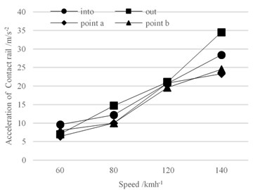
In addition, Fig. 30 gives acceleration of 4 feature points. As we can see, acceleration becomes larger when speed goes higher. Acceleration at 140 km/h is nearly twice acceleration at 120 km/h.

Throughthe analysis of contact force and vibration acceleration of sliding plate and conductor rail, when speed is over 120 km/h, the contact condition gets worse sharply which indicates that recommended speed for this electric shoegear and conductor rail system is 120 km/h.

Fig. 29Number of offline at different speeds

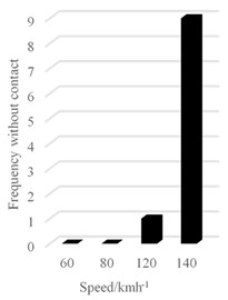
Fig. 30Vibration acceleration of conductor rail at different speeds

9. Conclusions

To treat conductor rail as a beam and electric shoegear as a cantilever, the author got vibration equations and vibration response matrix, solved the analytical modal coordinates by numerical integration and found the result that when speed increases, vibration of the rail and the shoegear both become more violent.

The author built up FEM model of electric shoegear. Stiffness of electric shoegear’s spring can be determined by vibration measurement.

Contact model of electric shoegear and conductor rail is established by penalty function method. Calculation result by using actual parameters shows the contact force change: decreases at first, and then re-decreases into a comparatively stable status after amplitude regaining.

Simulation results show that as speed goes higher, volatility of contact force increases. According to contact force and vibration acceleration of the rail and the shoegear, it is suggested that maximum operation speed of the system should be 120 km/h.

It should be noted that the present study is limited to the dynamics analysis for linear model of shoegears. A future study is expected considering nonlinear model of shoegears and the friction between the shoegear and the rail.