Abstract
The health status evolving from normal to broken condition of a milling tool is needed as an object of assessment in condition-based maintenance. This paper proposes continuous hidden Markov models (CHMM) to assess the status of the tool online based on the normal dataset in the same case. A wavelet-packet decomposition technology is used to feature extraction and the CHMM is trained by Baum-Welch algorithm. Finally, we compute the log-likelihood based on the trained CHMM for abnormal detection and health assessment in real time during the milling process. A case study on tool state estimation demonstrates the effectiveness and potential of this methodology.
1. Introduction
Tool wear in modern mechanical manufacturing systems, such as the milling process, is attracting considerable attention for the purpose of quality control. Tool conditional monitoring (TCM) ensures the accuracy of workpieces and reduces the costs caused by frequent replacement of the tools or process interruption. What’s more, it is essential to get the real-time wear state and feedback to the system to tune the milling parameters adaptively in modern automated and unmanned machining process. As a result, the design of TCM system has 2 requirements: (1) the algorithm has the ability of online health states determination and high accuracy; (2) the costs of system deployment should be as low as possible.
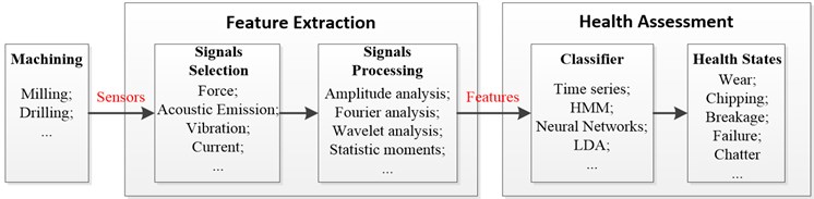
However, it is difficult to contact the health status and the wear severity. Tool wear is defined as the change in the shape of the tool from its original state during the operation process, which results in gradual loss of the tool material. Measuring the physical degradation variant directly, such as flank wear, is not flexible and is limited by the manufacturing equipment structure. Such measurement is difficult to conduct in the manufacturing process. Thus, the indirect methods focus on the features extracted from the signals of cutting forces, vibrations, acoustic emission (AE) motor/feed currents, and recognizing the dynamic undergoing health status through several data-driven models (i.e. neural networks, Time series) [1]. The flowchart of TCM can be summarized in Fig. 1. In general, the procedure includes two main parts: feature extraction and health status identification. The signals which may reflect the information about the tool wear are detected by the sensors. The features are vectors composed by some useful indicators extracted from the raw signals by many signal processing methods. Conventional signal processing methods include amplitude analysis, Fourier analysis, wavelet analysis, statistic moments and so on. After feature extraction, the health status of the tool is obtained by some classifier or cluster algorithms such as neural networks, Hidden Markov Models. These algorithms map the current features to a corresponding health status, i.e. normal, wear, breakage, failure for milling tools.
Among these models, the hidden Markov models (HMM) have been successfully applied to the condition monitoring of manufacturing machines [2]. The common usage often follows three steps. The first step is determining the degradation levels (i.e., good, partially worn, seriously worn, and broken) throughout the operating cycle. The second is constructing an HMM that would fit the degradation pattern and train the models. The third is selecting the HMM that, based on new incoming data, provides the highest likelihood of obtaining the actual degradation level [3]. Rabiner proposed another methodology that would train a single HMM by using the sensor measurements corresponding to the entire lifetime of the system, map each degradation phase to each state of HMM, and obtain the condition assessment by calculating the Viterbi path on new incoming data [4].
Fig. 1The systematic flowchart of TCM
This paper presents an online condition monitoring methodology of a milling process to determine the health status of the tool based on HMM and is aimed at reduce the requirement of training data in our models. The approach uses a continuous HMM to model one cutting pass and trains it by the data sampled under normal status of the working tool. Condition monitoring is performed by inputting a new observation sequence into the trained model and calculating the log-likelihood value that specifies the current health status from the normal one. The difference between our models and the conventional HMMs is that the conventional HMMs for TCM need features extracted from the specific wear stage to train the models, in the other words, one HMM for one wear stage. However, there are little sensor data, let alone lifecycle data for training the specific model in some cases. The proposed model works with training the HMM using data form the initial milling/cutting passes and estimating the variance between the initial milling/cutting “fingerprint” and the test one. Here the “fingerprint” is defined as the feature vectors from the sensor data.
2. Methodology
2.1. Signal processing and feature extraction
The reported methods for tool health assessment mentioned above are often based on sensing of the cutting forces, vibrations, AE, and motor/feed current mostly. These signals contain rich information about the condition of the tools. Zhu et al. trained a CHMM for modeling of the tool wear process in micro-milling, and estimation of the tool wear state given the cutting force features [5]. Pai et al. applied AE analysis for tool wear monitoring in face milling [6]. The fusion of multi-sensors information is also proposed to determine the health status of tools by integrating signals from multi-channels or different types of sensors, making TCM more accurate and comprehensible [7]. In the paper, we use signals of vibrations and AE to obtain the feature vectors.
Feature extraction is to find the indicators that can represent the actual tool wear process. Fourier analysis, time series and statistic moments are the general methodologies to get these indicators such frequency, Amplitude, RMS, kurtosis from the raw signals. Li et al. found that the amplitude of AE signals in frequency domain is very sensitive to the changes of tool status [8]. In order to obtain the enough frequency band range for both vibrations and AE signals, we choose wavelet packet decomposition (WPT) to extract features. Wavelet packet decomposition is a more elaborate signal processing method since it splits both approximation parts and detail parts to obtain a better frequency resolution. Suppose , , represent the original signal, approximation part and detail part respectively. In a commonly-used 3-level decomposition tree, the original signal is represented as +++++++ on the 3rd level and their frequency bands are 0-/16, /16-2/16, 2/16-3/16, 3/16-4/16, 4/16-5/16, 5/16-6/16, 6/16-7/16, 7/16-8/16, is the sampling frequency and /2 is the bandwidth [9].
What’s more, we also need to compute the wavelet energy which is the sum of square of detailed wavelet coefficients on each node for dimension reduction. The -th wavelet energy of coefficients on -th level can be defined as follows:
where is the wavelet coefficients of the -th node on -th level.
2.2. Continuous HMM and Gaussian mixture model
HMM is a popular tool in sequential data analysis since it has an interpretable mathematical structure which helps to form the theoretical basis required in different applications. It involves double-layer stochastic processes: the stochastic transition from one state to another and the stochastic output symbol generated at each state. All of the hidden states comprise a Markov chain through a set of transition probabilities between two states. The observation is assumed to be drawn from the state chain by the observation probability called emission probability. Thus, the actual sequence of states is hidden and not directly observable, whereas the observation sequence provides evidence to infer and determine the actual sequence of the states [5]. The complete specification of an HMM consists of the following elements:
1) a set of hidden states and initial state probability distribution expressed as:
2) transition probability distribution expressed as:
3) observation sequence which defines the individual observation sequence;
4) emission probability distribution expressed as:
which defines the distribution in state , and is the observation at time .
An HMM can be represented by the following compact notation to describe the complete parameter set of the model:
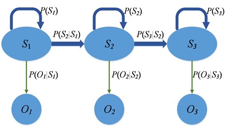
Numerous structures, such as ergodic HMM and left-right HMM, adapt to the specific problem [11]. From a physical point of view, we choose the left-right HMM to describe the milling process and set the HMM with three states: entry, in-progress, and exit.
In our case, the observation features extracted from the signals are continuous and the structure of HMM is designed to model the cutting process. Gaussian mixtures (GM) are typically used in continuous HMM (CHMM) to model the feature vectors that correspond to a state because of its variability and accuracy. The observation is modeled as GMM and expressed as:
where is the number of Gaussian functions, and are the mean and covariance matrix of each density function, and the weights are all positive and has a sum of one. The number of mixture components controls the accuracy of the emission matrix , and in turn influences the model. The Bayesian information criterion helps to determine the number based on the observations. However, selecting this number should consider the computation and efficiency.
Fig. 2A 3-state left-right HMM tool state assessment model
2.3. HMM algorithms
Three main problems are involved in implementing the HMM applications [12]. The issues we have to address in this study concerning the condition monitoring of tool wear are as follows:
1) estimation of the model to maximize , given the observation sequence .
2) evaluation of the probability of observation sequence , given the observation sequence and the model parameters .
The following two basic algorithms are proposed to solve the corresponding problems: the Baum-Welch algorithm and forward-backward algorithm. The former solves the problem of HMM training. This algorithm uses the observation sequence and adjusts the model parameters to maximize the probability , given an initialization of the model. The latter efficiently computes given a trained model and input observation .
3. Case study
3.1. Experimental setup
Given that the CHMM has the capability to model the dynamic character of the sequence, we train a single CHMM using the observations sampled in the normal pattern of the tool, and then send the observation sequence under an unknown wearing status into the normal-trained CHMM to compute the log-likelihood probability [10].
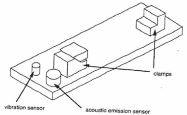
We used a mill dataset to test this condition monitoring methodology under one working condition which is accomplished by Kai Goebel (NASA Ames) and Alice Agogino (UC Berkeley) [13]. The data in this set represents experiments from runs on a milling machine under various operating conditions. In particular, tool wear was investigated in a regular cut as well as entry cut and exit cut. Data sampled by three different types of sensors (AE sensor, vibration sensor, current sensor) were acquired at several positions [13]. The setup of the experiment is as depicted in Fig. 3 and the layout of the sensors on the clamping device is shown in Fig. 4. An AE sensor and a vibration sensor are mounted to the table and the spindle of the machining center, respectively. The signals from all sensors are filtered and fed through two RMS before the data acquisition. The details of the experiment can be found in ref [14].
Fig. 3Experimental setup
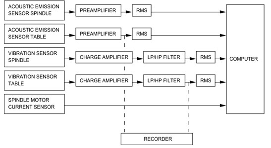
Fig. 4Clamping device with mounted sensors
To verify the proposed model of tool health status monitoring, we chose a test data set with long lifetime, its condition includes: speed run at 200 m/min, depth of cut at 1.5 mm, feed taken at 0.5 mm/rev, and material is cast iron. In this case, 17 runs are done with 9,000 samples in each cut.
3.2. Feature extraction
Fig. 5The observation sequence and feature vectors
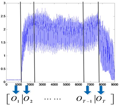
Signal preprocessing was performed to extract the features. We chose the signals of table vibration, spindle vibration, AE on the table, and AE on the spindle in one cut pass and extracted the features in frequency domain. The entire signal is sliced into 36 pieces with 250 samples in each piece. For each piece, a 3-level wavelet packet method was used to filter the noise and decompose these signals into three levels and obtain a vector consisting of the energy information in each frequency band, the structure of WPT is shown in Fig. 5 and Fig. 6. Different frequency bands had been proven to represent the effect of the force on different wear levels. Therefore each observation vector has eight wavelet packet energy values on each frequency band and the features are a sequence of 36 vectors, just like a fingerprint of the milling process.
Fig. 6A 3-level WPT of the signal
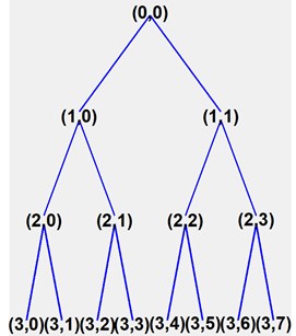
a) Tree decomposition
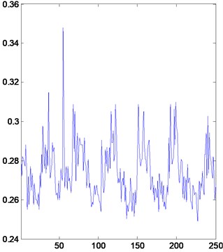
b) Data for node (0,0)
3.3. Construction of CHMM
The “fingerprint” of one process is constructed by wavelet-packet energy vectors. That is the observation sequence. To model this time series and recognize the state of this “fingerprint”, we chose a left-right CHMM and set the number of hidden states at three to represent the cutting pass with three successive states: entry, in-progress, and exit. The topology of the three-state left-right HMM is shown in Fig. 2. The transition matrix and the initial state of the left-right HMM are initialized as:
We assume that this online condition monitoring methodology can be implemented in a situation where the data are hard or expensive to acquire. The data from the first three run passes at the beginning are extracted to the feature vectors using wavelet packets transform as the “normal” dataset for model training. The emission probability distribution can be estimated through -means algorithm and GMM based on the training features. The CHMM is trained by the Baum-Welch algorithm. This algorithm uses expectation maximum to update the transition matrix A and emission distribution parameters base on the initial values in Eq. (7) by maximizing where is the number of training “fingerprints”. Here we use the first 4 cuts at the early stage of the lifetime in case 1 to train HMM and estimate the parameters of the model until the algorithm converges.
3.4. Online condition monitoring
Once the CHMM is trained, we can use this model to assess the health status of the tool through its lifetime. As the tool wears, the “fingerprint” will be more different from the normal one. The health status is defined based on the log-likelihood between the normal “fingerprint” and the wear ones, which is expressed as follows:
where is the “normal” model. We use the log-likelihood of the probability rather than the probability because the probability value may be so small that hard to distinguish the different health statuses intuitively. This value can be calculated by the forward-backward algorithm quickly. Thus, we input the feature sequence extracted from the data obtained under an unknown condition to the CHMM and compute the corresponding log-likelihood value that represents the current health status.
3.5. Experimental results
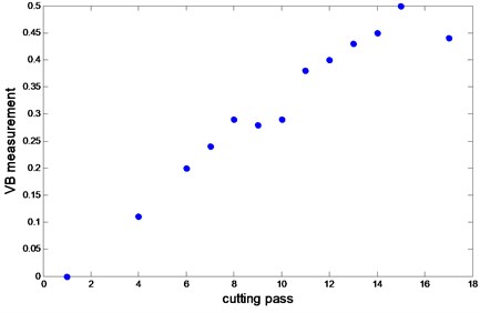
Due to friction of the tool on the work piece, the flank wear occurs and the wear VB is measured as the distance from the cutting edge to the end of the abrasive wear on the flank face of the tool in the experiments, shown in Fig. 7 [13]. As the tool wears, the VB measurement increases. All VB measurements of the flank in total 17 runs in this experiment are presented in Fig. 8.
Fig. 7Tool wear VB
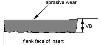
Fig. 8The VB measurements over the lifetime of the tool in case 1
In this paper, two different types of “fingerprints” are generated to train and assess the health status. One is the “fingerprint” only extracted from the signals of table vibration and spindle vibration, and the other consists of the features from table vibration, spindle vibration, AE on the table and spindle, making a mixed “fingerprint”. Then, we choose the “fingerprints” in the first three cutting passes as the training data and the subsequent fourteen ones as test data to perform health assessment. The log-likelihood value calculated by two different data types through the entire lifetime of the tool is shown in Fig. 9 and Fig. 10.
Fig. 9The entire trend of Log-likelihood obtained using only vibration signals
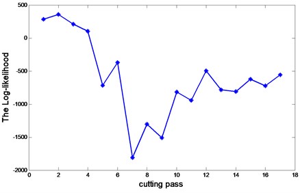
Fig. 10The entire trend of Log-likelihood obtained using both vibration and AE signals
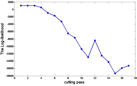
The experiment result indicates that as the flank wear VB increases, the log-likelihood value decreases over the entire lifetime of the tool. This finding means that the health status of the tool is moving far from the “normal” one. The results in Fig. 9 and Fig. 10 also show that the health trend obtained using vibration and AE signals is more reasonable than the health trend obtained using only vibration signals. The reason is that the degradation of the wear level is a gradual process. Another reason may affect the result is that the information of the vibration signals is not sufficient to express the actual health status of the tool. However, the features are not the more the better in consideration of the online deployment of the algorithm. It is crucial to find the features that could indicate the degradation of the tools.
4. Conclusion and future work
This paper presents an online condition monitoring methodology based on CHMM to assess the unknown health status of the tool. In the CHMM, the data from the normal status are used to train the model instead of the historical data, and the new observation sampled under the same case is sent into the model. The output of CHMM, log-likelihood of the probability, is considered as the index to quantize the current health status compared with the normal status. The results from vibration signals and combined signals are compared and demonstrate the importance of sufficiency of signal information. In addition, the improvement of the proposed methodology requires special adaptations to specific machining equipment or operating environment, such as setting failure thresholds, and the development of a universal and systematic approach is a definite objective of future research.
References
-
Kun Peng Zhu, Yoke San Wong, Geok Soon Hong Wavelet analysis of sensor signals for tool condition monitoring: A review and some new results. International Journal of Machine Tools & Manufacture, Vol. 49, 2009, p. 537-553.
-
Bjerkeseth M. Using hidden Markov models for fault diagnostics and prognostics in condition based maintenance systems. Ph.D thesis, University of Agder, 2010.
-
Peng Y., Dong M., Zuo M. J. Current status of machine prognostics in condition-based maintenance: a review. International Journal of Advanced Manufacturing Technology, Vol. 50, Issue 1-4, 2010, p. 297-313.
-
Rabiner L. R. A tutorial on hidden Markov models and selected applications in speech recognition. Proceedings of the IEEE, Vol. 77, Issue 2, p. 257-287.
-
Kunpeng Zhu, Yoke San Wong,Geok Soon Hong Multi-category micro-milling tool wear monitoring with continuous hidden Markov models. Mechanical Systems and Signal Processing, Vol. 23, 2009, p. 547-560.
-
Srinivasa Pai P., Ramakrishna Rao P. K. Acoustic emission analysis for tool wear monitoring in face milling. International Journal of Production Research, Vol. 40, Issue 5, 2002, p. 1081-1093.
-
Ai C. S., Sun Y. J., He G. W., Ze X. B., Li W. The milling tool wear monitoring using the acoustic spectrum. The International Journal of Advanced Manufacturing Technology, Vol. 61, Issue 5-8, 2012, p. 457-463.
-
Li Xiao, Li Yuan, Zhe Jun Tool wear monitoring with wavelet packet transform fuzzy clustering method. Wear, Vol. 219, 1998, p. 145-154.
-
Ekici S., Yildirim S., Poyraz M. Energy and entropy-based feature extraction for locating fault on transmission lines by using neural network and wavelet packet decomposition. Expert Systems with Applications, Vol. 34, 2008, p. 2937-2944.
-
Jianbo Y. Health condition monitoring of machines based on hidden Markov model and contribution analysis. Transactions on Instrumentation and Measurement, Vol. 61, Issue 8, 2012, p. 2200-2211.
-
Cartella F., Liu T. Online adaptive learning of left-right continuous HMM for bearings condition assessment. Journal of Physics: Conference Series, Vol. 364, 2012, p. 012-031.
-
Li Z., Wu Z., He Y, Fulei C. Hidden Markov model based fault diagnostics. Mechanical Systems and Signal Processing, Vol. 19, Issue 2, p. 329-339.
-
Agogino A., Goebel K. Mill Data Set, BEST lab, UC Berkeley. NASA Ames Prognostics Data Repository, http://ti.arc.nasa.gov/project/prognostic-data-repository, NASA Ames, Moffett Field, CA, 2007.
-
Goebel K. Management of uncertainty in sensor validation, sensor fusion, and diagnosis of mechanical systems using soft computing techniques. Ph.D Thesis, Department of Mechanical Engineering, University of California at Berkeley, 1996.
About this article

This research was supported by the National Natural Science Foundation of China (Grant Nos. 61074083, 50705005 and 51105019), as well as the Technology Foundation Program of National Defense (Grant No. Z132013B002).
