Bearing remaining life prediction using Gaussian process regression with composite kernel functions

1. Introduction

Bearings are the most widely used mechanical and rotational parts in industrial equipments [1]. In order to avoid the fatal breakdowns of machines caused by unexpected failures, defects of bearings should be detected as early as possible [2]. Condition based maintenance (CBM) which can reduce the cost of maintenance, becomes an efficient strategy for modern industry these years [3]. Effective prediction of bearing remaining life is important to identify the future conditions for maintenance plans, thus can reduce the downtime, maintenance cost and safety hazards [4].

Bearing performance prognostics means forecasting the remaining useful life (RUL) or future condition of equipment based on the acquired condition monitoring data. Although studies on prognostics of bearing RUL have received much attention recent years, the accurate estimation of the RUL of bearing is still challenging. Data-driven methods predict the results according to the historical records and the condition monitoring (CM) data. Vibration signal is effective to reflect the running condition of bearings [5]. Three major steps are crucial to achieve failure prediction result. Firstly, degradation indicator should be selected properly. Secondly, the degradation of machine should be tracked and assessed continuously. Finally, RUL of machine should be effectively predicted according to the monitoring data.

Prognostics algorithm is crucial to the effectiveness of failure prediction. Many popular prediction models have already been applied in the literatures. Artificial Neural Network (ANN) which has good self-learning and adaptive ability, is widely used in these prognostics models. In [6], Feed Forward Neural Network (FFNN) was used to achieve more accurate estimation of the RUL of bearings. Reference [7] proposed a recurrent wavelet neural network (RWNN) to predict the crack propagation of rolling bearings. Meanwhile, some new non-linear prognostics methods have also been employed to forecast RUL. For example, in [8], SVM-based model was developed to compute the ratio of bearing running time to failure time. In [9], a combination of logistic regression (LR) and relevance vector machine (RVM) was used to assess the health state and failure time.

These models work perfectly for some particular scenes. However, fewer machine learning methods can provide the probability density function (PDF) of RUL, which is important to handle the uncertainty problem. The probability indication of the predicted results is important to make maintenance decisions and risk analysis [10]. Sankalita Saha [11] proposed a distributed GPR-based prognostics algorithm to predict battery RUL with an uncertainty management. The results showed that GPR is superior to particle filters (PF) for battery prognostics.

GPR is a new promising technique which has received much attention in the machine-learning field over the past years. Due to the advantages in uncertainty predictions, GPR provides a good adaptability to handle nonlinear, complex classification and regression problems. Compared with artificial neural network, GPR is simpler to understand and implement in practice. Kernel functions in GPR models are similar with support vector regression (SVR) and relevance vector machines (RVM). However, GPR provides probabilistic outputs, by an uncertainty interval for the input data. Thus, GPR is being applied to various engineering problems with uncertainty.

Aiming to achieve an accurate failure prediction of bearing, a data-driven model based on GPR is proposed in this paper. A failure prediction model is constructed based on GPR with different covariance functions after feature extraction and fusion. The training input of this model is from bearings’ run-to-failure experiment.

The rest of the paper is organized as follows. In Section 2, GPR method is introduced detailedly. The bearing failure prediction model based on GPR is described in Section 3. In Section 4, applications of the proposed method are presented with experiment data. Finally, the conclusions are made in Section 5.

2. Principle of GPR

GPR is one of the most important Bayesian machine learning approaches [12]. As a probabilistic technique for nonlinear regression, it computes the posterior degradation estimates by constraining the priori distribution to fit the available training data.

Gaussian Process (GP) is a random process. It is defined as a series of random variables with any finite number of which has a joint Gaussian distribution. A GP is completely specified by its mean function $\mu \left(x\right)$ and covariance function $C(x,x\text{'})$, which can be defined as:

where $x\text{,}{x}^{\text{'}}\in X$ are random variables.

Given priori information about the GP and a set of training points $D=\left\{\left(x_i,f\left(x_i\right)\right)|i=1,2,\dots ,n\right\}\text{,}{x}_i\in R^d$ ($n$ is dataset number), the posterior distribution is derived by imposing a restriction on joint priori distribution [13]. A GP model with noise is defined as:

where $\epsilon$ is additive Gaussian noise $N(0,{\sigma }^2)$.

For a new test input $x^{*}$, we can establish a joint Gaussian priori distribution of the training output y and the test output $y^{*}$ as follows:

where $C\left(X,X\right)$ is $n$-order symmetric positive definite covariance matrix, $C\left(X,x^{*}\right)$ is the $n\text{×1}$ covariance matrix of the test input $x^{*}$ and the training input $X$, and $C\left(x^{*},x^{*}\right)$ is the covariance matrix of the test input $x^{*}$. Under the conditions of a given input $x^{*}$ and the training set $D$, the GP can calculate the test output $y^{*}$ according to the posterior probability formula as follows:

where ${\mu }_{y^{*}}$, ${\sigma }_{y^{*}}$ are expectation and variance of $y^{*}$ and $\alpha ={\left(C+{\sigma }_n^{2}I\right)}^{-1}y$, where $I$ is unit matrix.

The predicted mean value is a linear combination of covariance functions according to Eq. (7). A crucial ingredient in a Gaussian process predictor is the covariance function that encodes the assumptions about the functions to be learnt by defining the relationship between data points. Once a posterior distribution is obtained, it can be used to predict values for the test data points.

Three single covariance functions are used in this study, namely squared exponential (SE) covariance function, rational quadratic (RQ) covariance function and Matern class of covariance functions [12, 13]. These covariance functions are described as follows.

1) The squared exponential (SE) covariance function:

2) The rational quadratic (RQ) covariance function:

3) The Matern class of covariance functions:

where $\alpha$, $l$, ${\sigma }_f^2$, $M$ are hyper-parameters, and the $i$ and $j$ represent the $i$-th and the $j$-th vector in the input matrix $X$.

In order to predict the remaining life of bearing, GPR requires a priori knowledge about the form of covariance function. The choice of covariance function must be specified by users, and the corresponding hyper-parameters can be learnt from the training data. The parameters are optimized by maximizing the marginal likelihood algorithm [12], as shown in the following:

where $\theta =(\alpha ,l,{\sigma }_f^2,M)$ is a vector containing all hyper-parameters, and $Q=C+{\sigma }_n^{2}I$ is the covariance matrix for the noisy target $y$.

3. Remaining life prediction for bearings using GPR

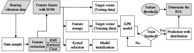
In this section, the remaining life prediction model is presented. The schematic diagram of the proposed model is shown in Fig. 1.

3.1. Feature extraction

Most mechanical failures can be represented by the feature of vibration signal. After feature extraction, several time-domain features can be obtained to assess the health state of the bearing and predict the RUL [14]. Three features are used in the proposed model, i.e. RMS, Kurtosis and Crest factor [15]. These features can be calculated as follows:

13

$Kurtosis=\frac{{\sum }_{k=1}^K{\left(x\left(k\right)-x_m\right)}^4}{K{x}_{std}^4},$

14

$RMS=X_{RMS}=\sqrt{\frac{\sum _{k=1}^K{\left(x\right(k\left)\right)}^2}{K}},$

15

$Crest=\frac{X_{PEAK}}{X_{RMS}},$

where $x\left(k\right)$ is a series of vibration signal for $k=$ 1, 2,…, $K$, and $K$ is the number of data points, and $X_{PEAK}$ is the maximum value of signal series.These features are usually stable under the normal condition, whereas they obviously change once bearings degrade. The three features are sensitive to different types of failures and the combination of them are more effective in performance assessment.

Fig. 1Schematic diagram of the proposed prediction method

3.4. GPR prediction

GPR is used to predict the failure time of bearings by assessing the features of bearings. The hyper-parameters are obtained by maximizing the marginal likelihood algorithm [13]. The model outputs the predicted MQE value and confidence interval for the next steps. The latest $k$ (in this paper, $k=$ 10) MQEs are took as input vector of GPR to predict the next several periods. The RUL of the bearing can be obtained based on the predicted MQE and failure threshold.

Covariance function is a key factor in GPR. Three standard covariance functions are used in this paper (i.e. squared exponential (SE) covariance function, rational quadratic (RQ) covariance function and Matern class of covariance functions). If $f_1\left(x\right)$, $f_2\left(x\right)$,…, $f_n\left(x\right)\mathrm{}$are independent random GP, $f\left(x\right)=\sum _{i=1}^n{f}_i\left(x\right)$ is also a GP. Therefore, a composite covariance function can be described as:

19

$C_{CK}\left(x^i,x^j\right)=\sum _{i=1}^n{C}_i\left(x^i,x^j\right).$

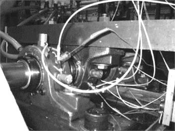
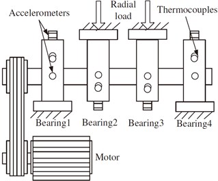
Fig. 2Bearing test rig sensor placement illustration

a)

b)

4. Case studies

In this section, we used the test data of bearing to validate the effectiveness of the proposed bearing failure prediction model. The bearing test dataset was generated from the run-to-failure test performed under a constant load condition by the national science foundation industry and university corporative research program (NSF I/UCR) center on Intelligent Maintenance Systems (IMS). The test rig is shown in Fig. 2.

Four bearings were installed on one shaft for the run-to-failure test [18, 19]. The rotation speed was maintained at 2000 rpm. A radial load of 2730 kg was placed onto the shaft and the bearings by a spring mechanism. Vibration data were collected every 20 minutes, with a sampling rate of 20 kHz. Three tests were carried out and all tests were terminated when some failure occurred.

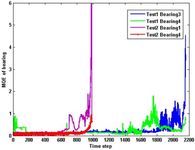
In order to give a brief demonstration of the proposed method, a part of MQEs were shown in Fig. 3. Three time domain features are applied to construct the input vector of SOM. After training SOM, the MQE of each test dataset can be calculated by Eq. (13)-(15).

Fig. 3MQE of test bearing

4.1. Prediction based on GPR

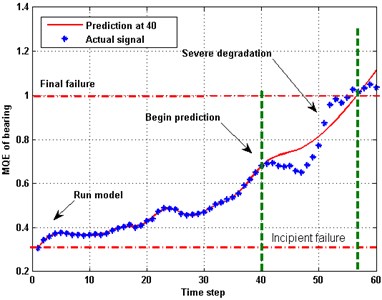
Several degradation datasets are extracted from Bearing 3 of Test 1 and used to make predictions. Performance degradation causes fluctuation of bearing vibration and the increase of MQE. When MQE exceeds the incipient threshold, the prediction model are activated. If MQE exceeds 1.0, bearing enters the failure stage and should be replaced.

The evolution of MQE of the vibration signal of bearing 3 with threshold setting and prediction is shown in Fig. 4. The prediction is trigged at the 40th time step, where the MQE is about 0.7. The dotted line is the actual MQE and the solid line indicates the prediction result of GPR with composite covariance function. The actual failure time is 55.3 and the predicted one is 56.6. The prediction is overestimated with an accuracy of 97.7 %, which is acceptable.

Fig. 4Remaining life prediction for bearing MQE

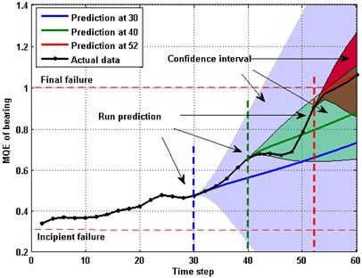
The prediction model based on GPR (CK) with 95 % confidence interval is used, as depicted in Fig. 5. Three prediction processes were triggered at the 30th, 40th and 52th time step, respectively. The corresponding MQEs of the bearing are approximately equal to 0.5, 0.7 and 0.9, respectively. The lines represent the predicted MQEs and the colored areas are the uncertainty areas of the predicted results. Among these lines, the black dot one indicates the actual MQE. It can be found that the predictions at 30 failed to follow the actual trend. Thus, prediction at the early stage faces a larger deviation. While, with more new data being added, the predictions become better as illustrated by the predictions at 40 and 52.

Fig. 5Prediction of MQE based on GPR (CK) with 95 % confidence interval at 30, 40 and 52

4.2. Comparisons between different kernels

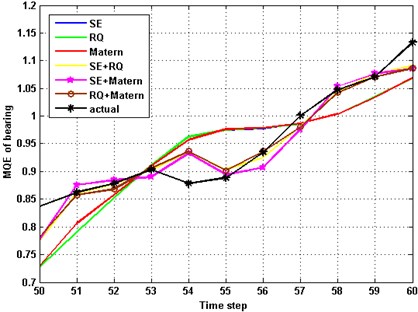
Covariance function is crucial for GPR, and can determine the efficiency of prediction. In this case, 60 points were used to make a comparison between different kernels. The length of the training data are 10. Six covariance functions are applied to the prediction model for training and validation. As shown in Fig. 6, most of kernels can suit the actual data well for one-step prediction. The RMS error (RMSE) and output variance are used to estimate the accuracy. Although, composite covariance functions consumed more time, they exhibited better performance (smaller RMSE and variance) than the single kernels. As listed in Table 1, the RMSE of the composite kernel of SE and Matern is smaller than others. Variance also reduces significantly. The composite kernel spent additional 60 % computing time in exchange for 30 % performance enhancement, which is valuable.

Fig. 6Predictions with different covariance functions

For an $n$-steps prediction, the dynamic of PDF predictions with single and composite covariance functions is shown in Fig. 7. The RUL distributions of both kernels cover the real RULs well. However, the distributions of RUL obtained from the single kernel have a larger PDF at early time, which means the variance of prediction is higher than the composite covariance functions. More accurate prediction with higher confidence can be obtained at the end life. This probabilistic implement help us make a correct judgment and provide an uncertainty management.

Fig. 7PDF of prediction with different covariance functions

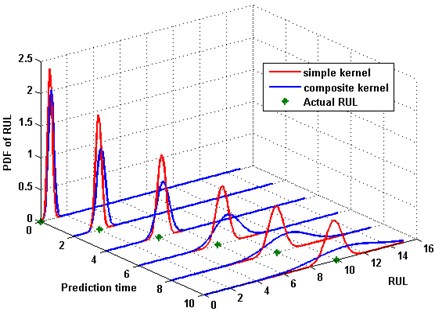
Table 1Comparison of different kernels

Kernel	RMSE	Variance	Computing time
SE	0.0357	0.08307	0.6738
RQ	0.0358	0.08290	0.9120
Matern	0.0351	0.08396	0.6930
SE+RQ	0.0197	0.03158	1.4845
SE+ Matern	0.0195	0.03515	1.0655
RQ+Matern	0.0190	0.03327	1.4503

4.3. Comparison with particle filter

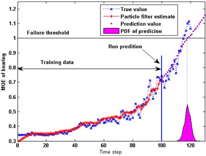
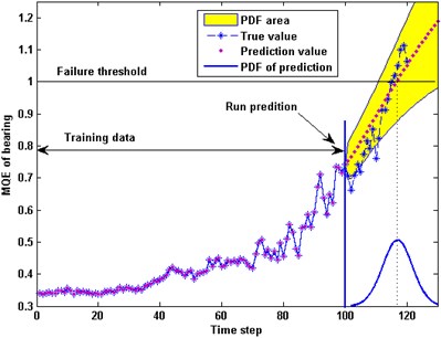
PF is a kind of Sequential Monte Carlo (SMC) methods that are coupled with the recursive Bayesian estimation [20]. The principle of PF is to utilize a set of weighted particles to represent the probability densities. 120 points degradation data are used to make a comparison. The failure threshold of the MQE is set as 1.0. The predictions are started at 100th time step. Both PF and GPR prediction model are run ten times and the average results are calculated. Fig. 8(a) is the prediction result using PF, and Fig. 8(b) is the prediction using GPR with the composite kernel.

Fig. 8Comparison of MQE prediction between composite kernel GPR and PF method

a)

b)

The actual failure time as shown in the Fig. 8 is 116.2. While the mean value of the predicted failure time by GPR and PF are 117.8 and 119.1 respectively. Both results are acceptable. Compared with PF, GPR has a better accuracy and the predicted curve of GPR is more stable. That is to say GPR is superior to PF in maintenance decision.

5. Conclusions

This paper proposes a bearing remaining life prediction model based on GPR with composite kernel. Dynamic of PDF is illustrated in the experiment. The PDF of model outputs is essential for risk analysis and maintenance decision. From this paper, following conclusions can be drawn:

1) This paper proposes a creative application of GPR in bearing prediction field. The GPR model can simplify the prediction process with a satisfactory performance.

2) GPR with composite kernels can improve the prediction accuracy and reduce the variance of the RUL in comparison with single kernel.

3) Compared with PF algorithm, GPR model is better in terms of prediction accuracy.