A hybrid prognostics approach to estimate the residual useful life of a planetary gearbox with a local defect

2.1. The dynamical model of the healthy planetary gearbox

Due to the multiple components and its orbital motion of the planets, the epicyclic stage of transmission system is more complex than the ordinary gear train. As the internal ring gear is fixed to the top of the transmission casing and the planet gear support is very rigid, the central displacement of the ring gear and the planet gears in the planetary gearbox can be ignored to simplify the model. Then a lumped parameter dynamical formulation is employed to develop the dynamical model of a common planetary gearbox. Deduced from Lagrange equations, the dynamical differential equations of this planetary gearbox could be listed as:

where ${\theta }_s$, ${\theta }_{pi}$ and ${\theta }_c$ denote the rotation angle of sun-gear, planet gear and carrier respectively. $T_D$ and $T_L$ denote the driving torque and the loading torque respectively. $r$ denotes radius and $r_b$ is the radius of basic circle. $m$ is mass, $I$ is the rotational inertia of subcomponents, for planet gear, sun gear and carrier, $I=1/2m{r_b}^2$. $N$ is the number of planet gear and $\alpha$ is the mesh angle. The subscripts $r$, $s$, $p_i$ and $c$ denote ring gear, sun gear, the $i$th planet gear and carrier. $D$ and $P$ is the adhesive engaging force and the elastic engaging force respectively.

Eq. (1) is positive semi-definite, nonlinear equations, which have $N+$2 degrees-of-freedom (dof’s). To translate the angle displacements of rigid bodies into the relative linear displacement, the relative displacement between the $i$th planet gear $x_{spi}$ and the sun gear, and the relative displacement between the carrier and the sun gear are defined as:

To simplify the model, the manufacturing errors and the mesh errors in the model are ignored as can be referred in [15]. After that, the internal meshing side clearance and the external meshing side clearance are defined as 2$b_{spi}$ and 2$b_{rpi}$, the adhesive engaging force $D$ and the elastic engaging force $P$ can be presented as:

where $K_{spi}$ denotes the mesh stiffness between the planet gear and the sun gear, $K_{rpi}$ denotes the mesh stiffness between the internal ring gear and the planet gear; $C_{spi}$ denotes the mesh damping between the planet gear and the sun gear; $C_{rpi}$ denotes the mesh damping between the ring gear and the planet gear. $K\left(t\right)$ is time varying mesh stiffness, and $f(x,b)$ is nonlinear clearance function, which is defined as:

where $b$ is the clearance constant.

After that, Eq. (2) and Eq. (3) are substituted into Eq. (1) and simplifying the equations, the dynamic model of 2K-H planetary gear set can be obtained. The equivalent mass is denoted as $M$, for the planet gear and the sun gear, $M=I/r_b^2\text{,}$ for the carrier, $M_c=I_c/{r_{bc}}^2+\sum _{i=1}^N{(m}_{pi}/\mathrm{c}\mathrm{o}{\mathrm{s}}^2\alpha )$.

2.2. The dynamical model of planetary gearbox with fatigue crack seeded

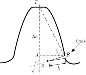
Fatigue crack is one of the common damages in planetary gearbox, and the cause of this damage is cyclic stressing of the gear tooth beyond its fatigue limit. Generally, the bending fatigue crack starts in the root section and it progresses until the tooth or part of it breaks off. The common fatigue crack occurs in the usual tooth root fillet section, so the tooth fatigue crack of sun gear is seeded in the model of planetary gear set in this section, as can be seen in Fig. 1.

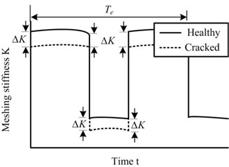
Fig. 1Gear-mesh stiffness variation of the gear pair with tooth crack

a)

b)

To simplify the model of damage, the shape of tooth root crack is approximated with straight lines, which are defined by the length l and the direction angle $\varsigma$ of the crack, as shown in Fig. 1. The level of crack is defined as $s$, which is determined by l and $\varsigma$, $s=s(l_j,\varsigma )$. For the mathematical tractability to solve the dynamical model, the crack size and its threshold value are defined as $c_j$ and $c_f\text{,}$$c_j=2m^{\mathrm{\text{'}}}\mathrm{c}\mathrm{o}\mathrm{t}\varsigma -l_j\mathrm{s}\mathrm{i}\mathrm{n}\varsigma \text{,}$${\tilde{c}}_j=c_j/c_f\text{,}$$j=$ 1, 2, 3,…. And then $s_j=s(l_j,\varsigma )=s\left({\tilde{c}}_j\right)$, $s_j\in \mathrm{}$[0 %, 100 %]. Referring [16, 17], the gear mesh stiffness of the gear pair is calculated by taking into account the geometric change due to the tooth crack. The details can be referred to [16].

The variation amplitude of gear mesh stiffness, which is caused by sun gear tooth crack, is defined as $\mathrm{\Delta }K(f_d,t)$, thus the time varying mesh stiffness of gear pair with tooth crack can be expressed as:

where $K_0\left(f_0,t\right)$ is the mesh stiffness of the healthy gear pair, $f_0$ is the mesh frequency, and $f_d$ is the meshing frequency of the gear pair with defect. $f_d$ is the function of the rotary frequency of sun gear $f_s$, the rotary frequency of carrier $f_c$ and the number of planet gears $N$, $f_d=N(f_s-f_c)$. The time vary mesh stiffness is illustrated in Fig. 1(b). The dynamical model of planetary gearbox with sun gear tooth crack is acquired by substituting Eq. (5) into the model deduced above.

2.3. Simulation of the dynamical models

The parameters in the dynamical model above should be set up according to Table 1. Parameter s is varied as [0 %:5 %:100 %] for the defect seeded model. Matlab 7.1 is used to execute this simulation, and four-order Runge-Kutta method is selected as the solution for the models. The step size and the duration for the solution procedure are set up to 0.0001 second and 1 second respectively.

The dynamic responses of the dynamical model in both the time domain and the frequency domain are shown in Fig. 2, which is for a healthy planetary gearbox ($s=$ 0 %) and 3 different levels of crack ($s=$ 20 %, 40 %, 80 %). The healthy model is characterized by the dominance of the gear mesh frequency, denoted by 1$X$ and its harmonics of 2$X$-6$X$, and etc. For the defect seeded models, the amplitude modulation in time domain of the gear mesh signal can be clearly observed, as can be seen in Fig. 2(a). As a consequence, many new frequency components appear at the left side of the dominant frequency (near 1/2$X$). The amplitude of the new frequency components increases with the growth of crack level, but the amplitude of dominant frequency and its harmonics decreases at the same time, as can be seen in Fig. 2(b). These features are very close to the experimental observations in the previous study literatures [16, 17, 21].

Fig. 2Dynamical response of the models

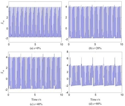
a) Time domain

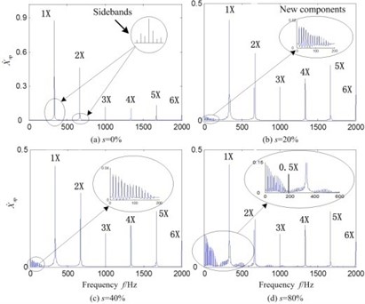
b) Frequency domain

2.4. Validation of the dynamical models

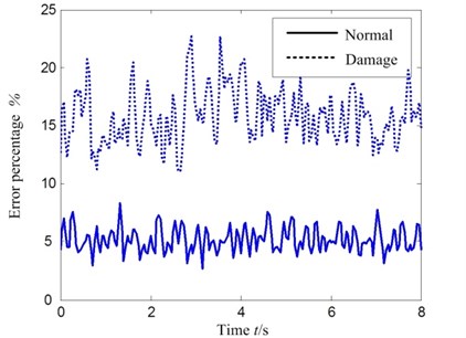
The test data sets in health condition and damage seeded condition are used to validate the dynamical model deduced in this paper. Above all, Root Mean Square (RMS) of each data set is calculated to reduce the effect of environment noise as the aid of the common algorithm TSA, and then the curves of error percentage of RMS between test data and simulation data of the dynamical models are depicted in Fig. 4. The real line is the error percentage between test data set and simulation data set in health condition, which is about 5 %, and the imaginal line is for damage seeded condition, which is about 15 %, as can be seen in Fig. 3. As the reason of that the damage seeded in the dynamical model above is simplified, which is different from the damage seeded in test. As a result, the imaginal line is above the real line obviously. Generally, the error percentage is low and the accuracy of dynamical model would be improved by considering more nonlinear factors of the damage seeded in the model.

Fig. 3Validation results of dynamical models

3.1. Feature selection

An optimal feature suitable for prognostics should have three merits: 1) Sensitivity, it means that the feature has a optimal classification distance; 2) Stability, which means the feature has the stable classification performance in different operation conditions (including loading and rotational speed). The target features will be selected from the 27 feature parameters above.

A statistic algrithm named two-sample Z-test is commonly used to measure the distance of two class samples [24, 27]. In this research, this algrithm is applied as sensitivity analysis algorithm, and then it is modified to analyze the stability and the relationality of feature parameters. The feature selection procedure can be described as follows:

1) Sensitivity analysis.

For the $k$th feature parameter, calculating the classification distance $Z_k$ of the healthy samples and the fault seeded samples under the identical operating condition by two samples Z-test procedure:

where ${\mathbf{X}}_1$ and ${\mathbf{X}}_2$ are the healthy sample set and the fault seeded sample set, $S_{\mathbf{X}}$ and $\stackrel{-}{\mathbf{X}}$ are the standard deviation and the mean of $\mathbf{X}$, respectively. And $n$ is the number of samples for each sample set. $k=$1, 2,...,$K$, $K$ is the number of feature parameters above. As the value of $Z_k$ increases, the sensitivity of the kth feature parameter will grow, that means the value of the $k$th feature parameter will have an obvious change while there is damage.

2) Stability analysis.

The classification distance of the kth feature parameter under the jth condition is defined as $Z_{k,j}$, $j=$1, 2,..., $J$. Then, the similarity ratio of classification distance for different condition, which is named stability in this research, is calculated:

where ${\mathbf{Z}}_k$ is the classification distance vector of the $k$th feature parameter for different condition, $Z_{k,m}$ is the mth element of ${\mathbf{Z}}_k$, $S_{{\mathbf{Z}}_k}$ is the standard deviation of ${\mathbf{Z}}_k$, $J$ is the number of operation conditions, $n$ is the element number of ${\mathbf{Z}}_k$. The numerator in Eq. (7) shows the general statistical characteristic of ${\mathbf{Z}}_k\text{,}$ and the denominator in Eq. (7) denotes the statistical diversity of classification distance of the $k$th feature parameter for different operation conditions. So $S_k$ indicates the stability of the kth feature parameter to different operation condition. As the value of $S_k$ increases, the stability of the kth feature parameter will rise, which means the $k$th feature parameter will keep stable while the operation condition (e.g. rotary speed and loading) changes.

According to the feature selection algorithms in this section, the feature parameter suitable for prognosis can be selected from the potential feature set when their evaluation criterion is predefined.

3.2. Feature weighting

As the feature vector includes more than one feature parameters, the feature weighting is necessary for fusing the analysis results of all the parameters in feature vector to achieve more reliable results. In this research, the weighting of feature parameter is determined based on the sensitivity and stability performance of the feature parameter calculated above. And also note that the weighting sum of all the feature parameters is equal to 1. Thus the parameters in feature vector can be weighted as follows:

where $i$ is the serial number of the feature parameter, $N$ is the number of feature parameter in the target vector.

4.1. Prognosis approach based on grey model

The simplest and most elementary form of grey model is GM(1,1) [31]. It is proposed as a forecasting model to extrapolate the original data sequence. The concept of the grey theory was first derived by Deng in 1986 [31]. It describes GM(1,1) model as approximations via least-square estimations at the first-order differential equation level. GM(1,1) has been widely used in the prediction of mechanical systems [31-38].

Vibration signal is an important information resource for monitoring rotary mechanicals. With the propagation of crack, the value of vibration indicators will increase generally. This process has two characteristics: 1) $X\left(t_i\right)\ge$ 0 and 2) $X\left(t_i\right)\ge X\left(t_{i-1}\right)$, which show the data set has strong tendency. These two characteristics meet the need to build grey model (GM), so GM(1,1) can be used to predict the future condition of planetary gearbox. The prediction procedure is as bellows:

Define $x^{\left(0\right)}=\left(x^{\left(0\right)}\left(1\right),x^{\left(0\right)}\left(2\right),\cdot \cdot \cdot ,x^{\left(0\right)}\left(n\right)\right)$ as the feature condition series, $x^{\left(1\right)}$ is the accumulated generating operation (AGO) of $x^{\left(0\right)}$, $x^{\left(1\right)}\left(k\right)=\sum _{i=1}^k{x}^{\left(0\right)}\left(i\right)$, $k\in \left\{1,\cdot \cdot \cdot ,n\right\}$; $z^{\left(1\right)}$is the mean generating operation of $x^{\left(1\right)}\text{,}$$z^{\left(1\right)}\left(k\right)=0.5x^{\left(1\right)}\left(k\right)+0.5x^{\left(1\right)}\left(k-1\right)\text{,}$$k\in \left\{2,\cdot \cdot \cdot ,n\right\}\text{.}$ GM(1,1) is:

The discrete model for prediction is:

where:

4.2. RUL estimation based on the modified grey model

To improve the prediction accuracy of the grey model in Eq. (10), a residual efficient $\epsilon$ is added to the grey input $u$ of the grey model for the addition of novel information from the physics-based models:

Then the discrete form is:

The residual efficient of feature $F_i$ is defined as ${\epsilon }_i$. After the feature parameters used for RUL prediction are determined, $\epsilon$ could be calculated based on the given information of simulation signal from dynamical model developed above:

where ${\widehat{x}}^{\left(1\right)}\left(1\right)$ and ${\widehat{x}}^{\left(1\right)}\left(k+1\right)$ are AGO of the time series of feature parameter $F$, and the elements of the time series are calculated based on simulation signal.

The one-step and multi-step prediction result of $F_i$ is $x_i^{\left(1\right)}\left(k+1\right)$, which could be obtained based on test data or real data according to Eq. (13). After that the value of prediction results $x_i^{\left(1\right)}\left(k+1\right)$ are fused utilizing the feature weight vector $W_i$ according to Eq. (15):

where $x_i^{\left(1\right)}\left(k+1\right)$ is the prediction result of $F_i$, and $W_i$ is the weight of $F_i$. Then $x_{}^{\left(1\right)}\left(k+1\right)$ in Eq. (15) is the expected value of future condition prediction.

In this research, RUL $N_f$ is expressed as the stress cycle of gear crack tooth $n$. $N_f$ is corresponding to $x_{}^{\left(1\right)}\left(k+1\right)$ according to Eq. (16):

where $\xi$ is determined based on the historical data of damage evolution test.

4.3. Description of the RUL estimation result

Logarithmic normal distribution (LND) is often used to describe the prognosis result of mechanical parts. In this research, the RUL probability distribution function of tooth fatigue crack in planetary gearbox is considered to belong to LND. The common form of LND is two-parameter-distribution, the density function is:

where $t$ is time, $\sigma$ and $\mu$ are the standard deviation and the mean, respectively.

As there are a lot of uncertainty issues in equipment operation, the accuracy of prediction result will decrease quickly while the prediction time extends, and then the variance of RUL distribution will grow. By iteration of modified grey model, multi-step prediction will be carried. Variance $\sigma$ could be expressed as the function of prediction life step $n$, $\sigma =\sigma \left(n\right)=\sigma e^{n-1}$. The RUL distribution is obtained by substituting the expressions of variance and expectation into Eq. (17):

Eq. (15) and Eq. (18) are combined, and then the prognosis result of tooth root fatigue crack in planetary gear sets is generated.

The relationship of RUL $N$ and failure time $T$ is correlated with operation profile in test/field, such as the rotary speed variation.

To evaluate the prognosis results, the prediction error $\eta$ is defined as the difference between the actual failure time $T_{af}$ and the predicted failure time $T_{pf}$:

where $T_{af}$ is the actual failure time, $T_{pf}$ is the predicted failure time and $T_c$ is the current time.

5.1. Test rig and the tooth crack propagation test

As can be seen in Fig. 4(a), the test rig provides torque and speed reduction through three stages, which simulates the main transmission system of general rotorcraft. The second stage is a planetary gearbox, of which the internal gear rig is splined to the top of gearbox casing.

To validate the prognostics approach in this research, a number of experiments have been conducted. The vibration signal generated by the planetary gearbox is picked up by an accelerometer bolted on the top of planetary gearbox casing and the electrical signal is transferred to the data acquisition system. The sampling frequency $fs$ is set up to 10 kHz. The signal is low-pass filtered at 2 kHz through a 4th order filter to limit aliasing distortion and retain waveform integrity of the effective signal. Data is stored in a PC for post processing. A number of 204,800 data points has been acquired in tests corresponding to a time-history length of 20 s.

In this research, an incipient crack is seeded in the sun gear, as can be seen in Fig. 4(b), and a run-to-failure test is carried out. In the test, the interval of sampling is 10 min. For every 50 minutes, the test is paused and the actual size of fatigue crack in propagation is checked. When the fatigue crack level reaches the threshold value, the test is ended. The threshold value of crack level is set up according to the experience of the prior test. The total run time of this crack seeded test is 736 min. From the test, the run-to-failure transitional data of fatigue crack propagation in sun gear of planetary gearbox is acquired.

Fig. 4Configuration of the test rig and the sun-gear with tooth root crack

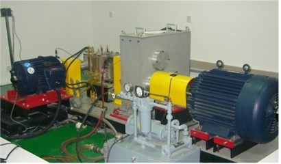
a) The test rig

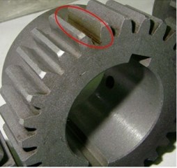
b) The sun-gear with tooth root crack

5.2. Validation results with test data

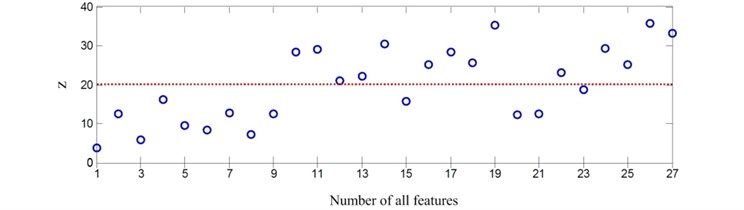
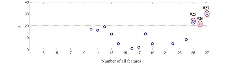
Based on the simulation data of the dynamical models, feature selection and weighting has been carried out before the test data validation. Only a few valueble features are kept and used, as can be seen in Fig. 5. As there is no prior knowledge of setting the threshold, a median value is used as selection criteria. In this research, [20, 20] is selected to be the threshold vector to illustrate the proposed methodology.

Fig. 5Feature selection results

a)

b)

In the feature selection procedure, the feature parameters are calculated based on the simulation data sets of the dynamical models with diferent level damge seeded. The procedure of the feature selection could be clearly dipicted in Fig. 5. The first step is the sensetivity analysis of feature parameters, the threshold value for this step is set up to 20, and the feature parameters #10, #11, #12, #13, #14, #16, #17, #18, #19, #22, #24, #25, #26, #27 are in the second step for stability analysis, as shown in Fig. 5(a). In the second step, the threshold value is set up to 20, and the selection result of this step is the feature parameters #25, #26 and #27, as shown in Fig. 5(a).

The feature parameters #25, #26 and #27 have been selected to be the remaining features, as shown in Fig. 5(b). These features are SK, LSK and NSR, and they are labeled $F_1$, $F_2$ and $F_3$ in this paper for convenience. Following the procedure in Eq. (9), the weights of these selected features are 0.2752, 0.2013 and 0.5235 respectively.

To validate the proposed RUL prediction approach in this research, the test data sets $X_1$~$X_4$ at time 360 min and 460 min are used for analysis. 50 feature samples of each test data set are extracted. The RUL for the test data at $t=$ 360 min and $t=$ 460 min is predicted. The prediction result of test data is recorded in Table 2, where $F_0$ denotes the healthy case, $F_t$ denotes the failure case, $F_A$ is the prediction result at $t=$ 360 min, $F_B$ is the prediction result at $t=$ 460 min. The RUL at $t=$ 360 min is 681 min with the confidence of 95 %. And the RUL at $t=$ 460 min is 705 min with the confidence of 95 %, while the real RUL of this test is 736 min.

According to Eq. (17), the prediction accuracy at $t=$ 360 min is 85.37 % and at $t=$ 460 min is 88.77 %. It could be seen from these prediction results that, as the prediction time reaches failure time, the accuracy of prediction result will be improved, in other words, the expected RUL of prediction result will approximate the real RUL, while the variance of prediction result decreases quickly. Compared to the traditional GM(1,1), the modified GM(1,1) has better accuracy and lower prediction error, which can be seen in Table 2.