The improved separation method of coherent sources with two measurement surfaces based on statistically optimized near-field acoustical holography

1. Introduction

Near-field acoustical holography (NAH) is a powerful tool that can reconstruct a three-dimensional (3-D) space sound field, i.e., sound pressure, particle velocity, and sound intensity, by propagating sound pressure data measured on a two-dimensional (2-D) measurement surface [1, 2]. Statistically optimized near-field acoustical holography (SONAH) has higher precision of NAH proposed by Hald to reduce the window effects associated with the spatial FFT used in conventional NAH [3-5].

A set of techniques about NAH have been developed to avoid the use of the discrete Fourier transform (DFT) [6], which more or less improve the computational efficiency and reduce the measurement data. There are several methods such as SONAH, inverse boundary element method (IBEM) [7, 8], and equivalent source method (ESM) [9, 10]. Partial field decomposition to identify the coherent sources by means of reference signal was proposed by J. Stuart et al., but it needed multi-reference microphones and to do continuous and more than once measurements [11]. Zhang et al. used orthogonal spherical wave put on maximum value of sound pressure over the sound source plane and double times calendar to confirm the source position, which would lose efficiency under the circumstance that interaction of multiple sources produced maximal values of pseudo sources [12]. Jerome made use of Bayesian theory to reconstruct the coherent sources and then obtained the source position by variable radius of a 2-D Hanning window, which also wasn’t suitable for the maximums of pseudo sources [13]. From the above discussion, those methods could all identify the coherent sources in some cases, but cannot be applied in any case.

Sound field separation technique with two surfaces makes a contribution to separate sound field information of the aim source from background noise [14-17], which applies a way to separate the coherent sources in the same direction of measurement surface. The present paper separates the coherent sources with two parallel measurement surfaces used improved method with SONAH, which would solve sources located at any position, reduce the measurement data and improve the computational time.

2. General underlying formulation

2.1. Theory of SONAH

Basic theory of SONAH: Assume that complex time-harmonic sound pressure $p\left({\mathbf{r}}_i\right)$ has been measured in free and homogeneous region $\mathrm{\Omega }$ by a set of positions ${\mathbf{r}}_i$, $i=\text{1, 2,…,}N$. The amplitude and phase of each elementary wave in the sound field is written as:

1

$p\left({\mathbf{r}}_i\right)=\sum _{m=1}^M{a}_m{\mathrm{\Phi }}_m\left({\mathbf{r}}_i\right),i=1,\dots ,N.$

Here, $a_m$ are the complex expansion coefficients. When $N\ge M$, the $a_m$ can be calculated by the least-squares equivalent wave model. There are $M$ wave functions, ${\mathrm{\Phi }}_m$, measured at $N$ hologram locations.

Generally, the elementary waves are plane and evanescent, and they are considered to be a free-field condition. Sources behind a source plane, radiate into the source free, homogeneous half space. When sources are not restricted to a half space, as illustrated in Fig. 1, where measurements are taken in a free and homogeneous source field between two parallel source planes, $z_0^{+}\le z\le z_0^{-}$. In this space, the radiated sound field can be represented by plane wave functions of the combined set:

2

${\mathrm{\Phi }}_{\mathbf{k}}^1\left(\mathbf{r}\right)=e^{-j\left(k_{x}x+k_{y}y+k_z\left(z-z_0^{-}\right)\right)},$

3

${\mathrm{\Phi }}_{\mathbf{k}}^2\left(\mathbf{r}\right)=e^{-j\left(k_{x}x+k_{y}y+k_z\left(z-z_0^{+}\right)\right)},$

where $z_0^{-}$ and $z_0^{+}$ are source positions in $z$ axis, $\mathbf{r}=\left(x,y,z\right)$ is a position vector, and $\mathbf{k}=\left(k_x,k_y,k_z\right)$ is a wave number vector with:

4

$k_z=\left\{\begin{array}{c}\sqrt{k^2-\left(k_x^2+k_y^2\right)},\left(k_x^2+k_y^2\right)\le k^2,\\ -j\sqrt{\left(k_x^2+k_y^2\right)-k^2},\left(k_x^2+k_y^2\right)>k^2.\end{array}\right.$

Matrix $A$ is the formulation of wave function values at the measurement positions, defined as:

5

$\mathbf{A}=\left[\begin{array}{c}\begin{array}{cc}{\mathrm{\Phi }}_1\left({\mathbf{r}}_1\right)& {\mathrm{\Phi }}_1\left({\mathbf{r}}_2\right)\end{array}\begin{array}{cc}\cdots & {\mathrm{\Phi }}_1\left({\mathbf{r}}_N\right)\end{array}\\ \begin{array}{cc}{\mathrm{\Phi }}_2\left({\mathbf{r}}_1\right)& {\mathrm{\Phi }}_2\left({\mathbf{r}}_2\right)\end{array}\begin{array}{cc}\cdots & {\mathrm{\Phi }}_2\left({\mathbf{r}}_N\right)\end{array}\\ ⋮⋮\begin{array}{cc}\ddots & ⋮\end{array}\\ \begin{array}{cc}{\mathrm{\Phi }}_M\left({\mathbf{r}}_1\right)& {\mathrm{\Phi }}_M\left({\mathbf{r}}_2\right)\end{array}\begin{array}{cc}\dots & {\mathrm{\Phi }}_M\left({\mathbf{r}}_N\right)\end{array}\end{array}\right].$

Vector $\mathbf{p}$ and the matrix $\mathbf{\alpha }\left(\mathbf{r}\right)$ at reconstruction positions can be written by the following form:

6

$\mathbf{p}=p\left({\mathbf{r}}_i\right)=\left[\begin{array}{c}p\left({\mathbf{r}}_1\right)\\ p\left({\mathbf{r}}_2\right)\\ ⋮\\ p\left({\mathbf{r}}_N\right)\end{array}\right],\mathbf{}\mathbf{}\mathbf{}\mathbf{\alpha }\left(\mathit{r}\right)=\left[\begin{array}{c}{\mathrm{\Phi }}_1\left({\mathbf{r}}_s\right)\\ {\mathrm{\Phi }}_2\left({\mathbf{r}}_s\right)\\ ⋮\\ {\mathrm{\Phi }}_M\left({\mathbf{r}}_s\right)\end{array}\right],$

here, ${\mathbf{r}}_s$ is a position vector at the reconstruction locations.

To obtain the pressure at the reconstruction location, $p\left({\mathbf{r}}_s\right)$, we use Tikhonov regularized solution to resolve the single value which would come out during the inverse operation of matrices. After a set of calculation, $\mathbf{p}\left({\mathbf{r}}_s\right)$ is given by:

7

$\mathbf{p}\left({\mathbf{r}}_s\right)={\mathbf{p}}^T{\left({\mathbf{A}}^H\mathbf{A}+\epsilon \mathbf{I}\right)}^{-1}{\mathbf{A}}^H\mathbf{\alpha }\left(\mathit{r}\right),$

where ${\mathbf{A}}^H$ is the conjugate transpose of $\mathbf{A}$, $\mathbf{I}$ is a unite diagonal matrix and $\epsilon$ is positive regularization parameter, provided by Hald [4], is given by:

8

$\epsilon =\left(1+\frac{1}{{\left(2kd\right)}^2}\right)\bullet {10}^{-\frac{SNR}{10}},$

where $SNR$ is the signal to noise ratio including random error and noise, and $d$ is the distance between measurement surface and reconstruction surface.

Fig. 1Two parallel source planes limiting a homogeneous and source-free region

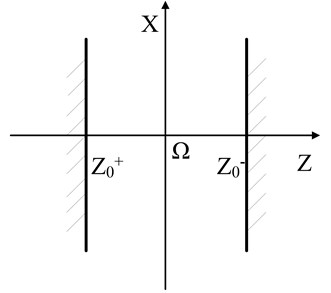
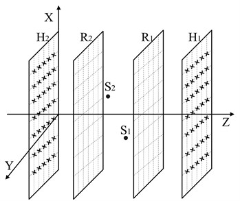
Fig. 2The positions of measurement surfaces, reconstruction surfaces and sources

3. Numerical simulations

According to the set-up illustrated in Fig. 2, a set of measurements were simulated. There, the grid shows an 8×8 element microphone array with 6 cm grid spacing, the microphone being at the corners of the grid. The centers of two coherent in-phase monopole point sources of equal strength are located at (–0.15, 0, 0.11) m and (0.15, 0, 0.06) m, respectively. The distance between measurement surface $H_1$ and source point $S_1$ was 0.06 m, the distance between measurement surface $H_2$ and source point $S_1$ was 0.11 m, and the gap between the two measurement surfaces was 0.17 m. SONAH calculations were executed in the measurement surfaces and construction surfaces. The calculation grid in the construction surfaces had the gird by 13×13 data points with the same grid spacing as measurement grid. The regularization parameter in Eq. (8) was set to 40 dB according to $SNR$, and the source distance $d$ was set to 0.06 m. In addition, the relative average error level during calculation proceeding was given by the formula:

where $L_{err}$ is the relative average error level and $p_i^{ture}$, $p_i$ are the truth value of pressure and the calculation value of pressure, respectively.

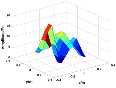
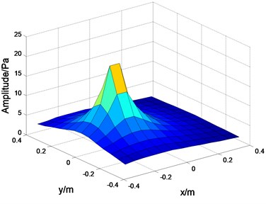
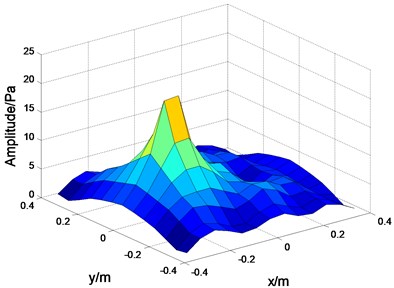
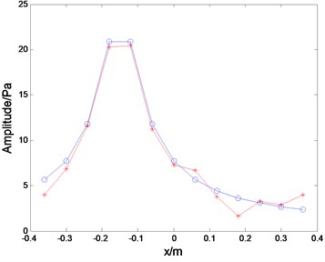
Fig. 3Pressure amplitude: a) the measurement surface H1; b) theoretical value on reconstruction surface R1; c) calculated value on reconstruction surface R1; d) comparison section view on xoz plane

a)

b)

c)

d)

At first, a simulation at a single frequency of 1000 Hz was investigated, i.e. the aim to separate the source point $S_1$ from the coherent sources.

Figs. 3(a)-3(d) depict the pressure amplitude of measurement surface $H_1$, theoretical value of reconstruction surface $R_1$, calculated value of reconstruction surface $R_1$ and comparison sectional view of theoretical and calculated value in reconstruction surface $R_1$, respectively.

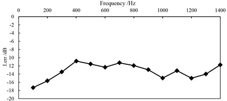
Fig. 4Relative average error level of SONAH calculation for pressure in the reconstruction surface

After the sound field separation process, Fig. 3(b) shows the good agreement with the theoretical value depicted in Fig. 3(c). Here, the relative average error is –14.98 dB. It is obvious that, by using the improved sound field separation technique with SONAH, the pressure produced by a single source from the coherent sources on the measurement surface $H_1$ can be separated out correctly.

In order to further verify the performance of sound field separation technique with SONAH, the relative average errors at different frequencies (from 100 Hz to 1400 Hz) were studied by simulation. Fig. 4 shows the relationship between frequency and relative average error. Here, the relative average error is all below –10 dB, which is acceptable.

4. Practical measurement

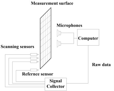
A practical measurement to examine the method proposed in this paper was conducted. The set-up consisted of two loudspeakers radiating steady sound field with 1000 Hz as two coherent sources. Other instruments were set according to simulation conditions. Figs. 5(a) and 5(b) indicate the schematic diagram and photo of the experimental setup.

Fig. 5Experimental setup: a) the schematic diagram; b) practical photo

a)

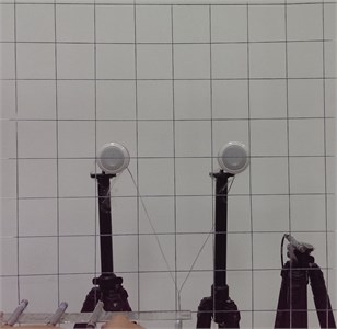
b)

Fig. 6Reconstruction result: a) three-dimensional diagram; b) contour plot

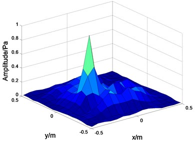
a)

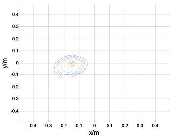
b)

The pressures of time domain on the two measurement surfaces were measured by a scanning microphone composed of 3 microphones a few times and a fixed reference microphone. Every measurement surface puts 81 measuring points, which were composed of 3 microphones with 27 times, respectively. During the whole mensuration, the reference microphone collected the data as the 3 microphones all the way. Then, the complex pressures of measurement surfaces were calculated by the measured data and reference data. The amplitudes of pressures and the phased of pressures were got through FFT transform, further, the phase differences of pressure were calculated. According to the amplitudes and phase differences of pressure, the complex pressure data were worked out.

Figs. 6(a) and 6(b) show that the position of target source $S_1$ on the reconstruction surface $R_1$ is same as the position on the measurement surface $H_1$ and $S_1$ is completely separated from the coherent sources, although there are some errors, which do not disturb the recognition of the target source that is needed to be identified.

5. Conclusions

The improved sound field separation method of coherent sources based on statistically optimized near-field acoustical holography has been proposed and examined in this paper. The method, based on the measurement of pressures in two parallel layers and reconstruction of pressures on the measurement surfaces, respectively, makes use of the relationship between data on the measurement surfaces and on the reconstruction surfaces to separate the single source from coherent sources. This method could not only reduce the measurement data, but also improve the computational accuracy. Their performance in the sound field space has been examined numerically and experimentally.

This separation method of coherent sources would obtain the sound field information of single source, which avoids the interference of other sources with the same frequency. In practical applications, such method could locate the source position more precisely and identify the size of source more accurately.