Abstract
Evaluating structural damage, caused by earthquakes, is very important in seismic risk management. Zoning maps of structural damage are directly used in evaluating damage of different zones as well as planning to retrofit structures. Attenuation relation is applied in preparing the acceleration zoning of regions. Similarly, damage attenuation relations which are used in analyzing probabilistic hazard and preparing damage zoning are obtained by structural damage spectrum. This spectrum is nonlinear and designed by considering nonlinear parameters of a series of one-degree-of-freedom structures and time history dynamic analysis. After gathering and modifying 778 records of the earthquakes happened in Iran, the damage spectrum was prepared for X-braced steel structures with different specifications (yield force, hysteresis curves, and ductility capacity). Damage attenuation relation was developed for the structures through regression analysis and the obtained results were compared with those of artificial neural network method. Damage of three samples with different specifications was calculated by the developed attenuation relation. The obtained results were compared with those of time history dynamic analysis. The developed relations were used for analyzing the probabilistic damage risk and preparing the damage zoning maps for city of Qazvin, as a seismic region in Iran.
1. Introduction
Different seismic parameters such as base design acceleration, site specific design spectra, and earthquake records are needed in dynamic analysis of structures. An ordinary method for calculating base acceleration is based on earthquake hazard analysis. In this method, base acceleration and design acceleration are obtained based on the seismicity of the region, site condition, and spectral attenuation relation as well as using probabilistic methods. These parameters can be used in the analysis of structures. Then, structural damage is calculated using the results obtained from structural analysis. On the other hand, damage spectrum and damage attenuation relation can be directly computed in order to calculate the damage of a structure in a certain region, instead of calculating the acceleration spectrum or velocity. However, before analyzing the damage risk for a certain region, it is necessary to have its attenuation relation. Many attenuation relations have been prepared for acceleration, acceleration spectrum, etc. Based on the logic of producing these relations, damage attenuation relation is provided for a specific region. Attenuation models have a half century history. These models have been primarily provided very simply and based on limited parameters such as magnitude and distance. They have been evolved over time and are now converted into complex models considering different parameters such as magnitude, distance, tectonic condition, soil type, etc. Besides their complexities, attenuation models have become more accurate owing to development of computer science and based on probabilistic statistical analysis. In this study, first, seismic information of the region was gathered and then the attenuation relation was provided for damage spectrum of steel structures.
With respect to the limited damage attenuation relation available in the literature, a brief history of attenuation relation, related to the acceleration, is presented in this section. No information can be found in the literature before Newman's research in 1954, who presented the attenuation model of strong ground motion acceleration based on the earthquakes of America and their accelerograms in the form of a relation of distance, independent from magnitude. In 1970-1980 and particularly after the event of Sanfernando in California, more attenuation models have been presented with many accelerograms of the accelerations of this earthquake by the researches such as Milne and Davenport (1969), Esteva (1970), Donovan (1973), Esteva and Villaverde (1973), Orphal and Lahoud (1974), Ambraseys (1975), Trifunac (1976), and Cornell et al. (1979). All these models have used the earthquake data and accelerograms of western America, particularly California. The magnitude of earthquake and its focal distance from acceleration (or other parameters) recording stations have been used in the presented models. The applied earthquake magnitudes have been 4-7.7 and the distances between accelerograms and focal point have been 5-300 km [1]. Since 1980, the parameters of attenuation models have been calculated more accurately owing to the availability of accelerogram data. Moreover, uncertainty has been considered in the calculation using mathematical methods. These attempts have resulted in the attenuation models, in which the geotechnical conditions and earthquake mechanisms have been considered. Some specifications of the models, presented since 1980, are mentioned below.
The attenuation model presented by Battis [2] was based on the earthquakes of California with the magnitudes of 5-6.5 and distances of 10-350 km. He has presented another model based on the earthquakes of central America with different conditions as well.
Campbell [3] presented his attenuation model based on the world's earthquakes with the magnitudes of 5-7.7 and distance of less than 50 km from strong ground motion acceleration recording stations. The model was related to rock and soil sites with the thickness of over 10 km.
The attenuation model by Joyner and Boore [4] was provided based on the earthquakes of northwest of America with the magnitudes of 5-7.7 and distance of 370 km from strong ground motion acceleration recording stations. The model had some factors which can estimate accelerations for soil and rock conditions.
Boor and Joyner [5] provided their attenuation model based on the earthquakes of western America for soil and rock sites considering earthquake magnitudes as ML and different distances.
The attenuation model by Joyner and Boor [6] reviewed the previous models to get more information about the earthquakes of northwest of America.
The attenuation model by Boor and Atkinson [7] provided an assessment of the earthquakes of northwest of America with moment magnitudes of 5.0 7.0 and distances of 10-100 km from strong ground motion acceleration recording stations. In this model, the focal depth was considered 10 km.
Change in the processing of attenuation model has been basically started since 1980. The last attenuation models were presented in the proceedings of a specialized workshop, “Strong Ground Motion in California”, which was held in December 1993. They were presented internationally and provincially, particularly in the regions of seismic countries.
Douglas gathered and classified a complete complex of a large part of acceleration attenuation relations and response spectra of the world since their beginning. This complex information was used for obtaining new attenuation relation [8]. Some specifications of the models presented since 2003 are mentioned below.
The attenuation model by Bragato and Slejko [9] was provided based on many data and records of Eastern Alp earthquakes with the magnitudes of 2.5 6.3 and distances of 130 km.
Ghodrati Amiri, Mahdavian, and Manouchehri Dana [10] attempted to derive attenuation relationships for PGA, PGV, and EPA parameters for areas within the seismic zones of Zagros Alborz and Central Iran with rock and soil sub-structures. To do so, at first, the available scientific data including the methods used for deriving attenuation relationships and the involved parameters were gathered. Afterwards, all the efforts were focused on gathering a thorough catalogue of earthquakes occurred in Iran. In this regard, the majority of the available catalogues in Iran were gathered and corrected though different methods. Finally, a set of 89 earthquake events including 307 earthquake records with reliable data was chosen.
The development of strong ground motion models used in the zoning of Italian earthquakes was provided using 922 records of 116 earthquakes with the magnitudes of 4-4.5, recorded in 137 stations, and distance of 100 km from the epicenter [11].
The NGA-West2 [12] project was a large multidisciplinary, multi-year research program on the Next Generation Attenuation models for shallow crustal earthquakes in active tectonic regions. This research project was coordinated by Pacific Earthquake Engineering Research Center (PEER) with extensive technical interactions among many individuals and organizations.
Damage attenuation relationship based on damage spectrum concept was developed by Bozorgnia and Bertro [13], who conducted nonlinear dynamic analysis on single degree of freedom (SDOF) structures with constant specifications such as period, damping ratio, strength, soil site condition, and force-deformation using an earthquake record. Then, damage values of single degree of freedom structures, subjected to earthquake record, were calculated using hysteresis curves obtained from dynamic analysis and selecting an appropriate damage function.
A procedure similar to the aforementioned ones can be used for finding the rates of structural damage in certain sites, instead of calculating acceleration. Damage attenuation relation can be obtained using the logic followed in other studies for accessing the acceleration attenuation relations. Damage spectra of structures should be plotted for obtaining damage attenuation relation. As in the classic methods, several single degree of freedom structures have been considered for gaining damage spectrum.
By using acceleration spectrum preparing algorithm and selecting an earthquake record, nonlinear dynamic analysis was conducted for different nonlinear parameters. Damage spectrum was prepared using the results of nonlinear dynamic analysis of the parameters such as maximum displacement, hysteresis energy, etc. Therefore, the obtained damage spectrum was affected by the selected damage function. Different damage functions and the one applied in this research are presented below.
2. Damage index
There are different kinds of structural damage functions; but, Krawinkler damage index is mostly used in steel structures, as all tests, performed for calibration its relation have been conducted on I-form steel sections. According to this index, many tests have been conducted on two main groups, each containing 10 samples. The samples are subjected to uniform loading, cyclic loading with constant deflection, and cyclic loading with varying deflection.
The main relation of Krawinkler index is defined as Eq. (1):
where, ; is the number of damage cycle, , , , and are structural damage parameters, is plastic deformation in the ith damage cycle, is damage, and is the number of cycles up to failure.
The following assumptions have been considered in calculating this index.
The relation between the number of cycles up to failure () and plastic deformation is calculated according to the studies by Monson Coffin and expressed as Eq. (2):
Miner’s relation has been used to consider the earthquake cumulative effects, in which damages is linearly summed and defined as Eq. (3):
Small deformations have been ignored, as they have a slight effect which is entered through high cycle fatigue theory, concerning the relative cycles of earthquake [14].
A damage function should be selected and used for designing the damage spectrum. In this study, Krawinkler damage function was used.
3. X-braced frame simulation
In this project, OpenSees software was used for identifying hysteresis (cyclic simulation) and modeling X-braced low fatigue. This software, with a rich library of material, sections, structural and geotechnical elements, solution algorithm, etc., is applied for structural and geotechnical simulation. In order to simulate X-braced cyclic behavior, a model including steel element (Steel02) was applied [15, 23]. This element uses uniaxial Giuffre-Menegotto-Pinto model along with isotropic hardening. Fig. 1 shows the hysteresis behaviors of single- and X-braced samples subjected to quasistatic time history loading. Fiber elements and low eccentricity (1/1000 of element length) were applied in order to provide buckling capability for bracing elements. Moreover, to provide out of plane buckling, a single degree of freedom braced frame was modeled three dimensionally. Eccentricity was applied either out of plane or in plane. Therefore, the braces had out of plane and in plane bucklings.
Fig. 1Quasistatic analysis for single braced and X-braced frames

a) Quasistatic time history

b) X-braced frame
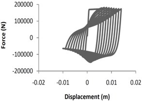
c) Single braced frame
4. Damage spectrum
Damage spectrum of the considered record can be plotted by repeating the above mentioned process for single degree of freedom structures with different periods (Fig. 2).
As shown in Fig. 2, a record should be selected to prepare damage spectrum in the first step. Then, a single degree of freedom system with a specific period is selected and level of ductility is determined. Afterward, to determine nonlinear characteristics of the structure such as chart mentioned, can use of code or with respect to structural vulnerability, appropriate ratio of yield stress to weight is selected. Using nonlinear dynamic analysis, the response of the structure of single degree of freedom is obtained and, in the next step, by choosing a suitable damage function and response analysis, damage of the single degree of freedom structure is achieved. By repeating the above steps for the structures with single degree of freedom with different periods, damage spectrum is drawn. So, damage spectrum is obtained for various records. Definitely, the given spectrum is concerned to nonlinear properties. Also, damage spectrum obtained from the above steps is affected by the choice of a suitable damage function. In other words, the spectrum of acceleration, velocity, and displacement can be plotted for a certain record. Similarly, the damage spectrum can be also drawn by a certain record and period range. The record catalogue used in this study was related to Iran and included 772 earthquake records (Fig. 3).
Fig. 2Damage spectrum designing steps
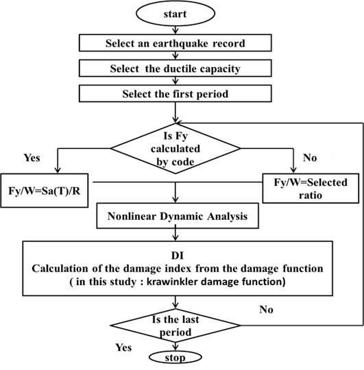
Fig. 3The specifications of gathered records
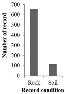
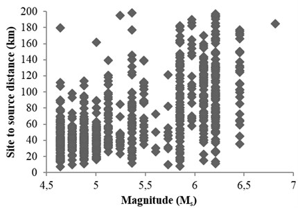
Since the purpose of this study was to obtain an attenuation damage relationship for the Iranian plateau zone, therefore, time histories of Iranian plateau (recorded in Iranian Building and Housing Research Center) were used [16]. Although the number of data recorded in Iran was more than two thousand and the number of reliable records with geological properties was limited, so 772 records were selected. 116 records were related to soil condition and 565 others were related to rock conditions. Also in this study, the magnitude of records was between 4.5 and 7 and site to source distance was between 10 and 200 km.
As mentioned in the earlier sections, Giuffre-Menegotto-Pinto steel material object with isotropic strain hardening was used in this research. Nonlinear force-displacement parameters are needed for dynamic analysis and damage index calculation. In this regard, yield force is considered in 6 different states. In states 1-5, the ratio of yield force to weight () is assumed constant for all periods in a certain damage spectrum as 0.05, 0.1, 0.15, 0.2, and 0.3, respectively. Moreover, as a building in Iran may be designed according to the Iranian Codes [17], the yield force might be about the base shear. Therefore, ratio is obtained from Eq. (4) for state 6:
where is spectral acceleration, is redundancy factor, is yield force or base shear, and is weight of structure. Assuming that the ultimate displacement is needed in the nonlinear analysis of structures and calculating the damage values, displacement can be expressed as a coefficient of yield displacement. This coefficient is called ductility capacity. As the results obtained in this research were used for studying the damage of buildings in Iran, ductility value was calculated according to Iranian Codes. Therefore, the ductility values were considered as 2, 3.5, and 5 for X-braced steel structures with ordinary, intermediate, and special ductility, respectively.
Concerning the above explanations as well as the way of damage spectrum designing shown in Fig. 2, the damage spectrum was plotted for 6 states of ratio, 3 states of ductility capacity, and 772 records. In other words, in total, 13896 states were designed, some examples of which are shown in Figs. 4 and 5, which were based on theoretical analysis and was done by Matlab programming and OpenSees modeling.
Fig. 4Shirinsoo earthquake: mb= 6.2 -R= 57 km; rock condition; Ordinary ductile
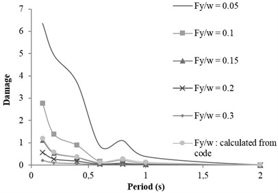
Fig. 5Bandargaz earthquake: mb= 5.6 -R= 52 km; soil condition; Special ductile
5. Attenuation relation of damage spectrum
The main stage in forming the predicting relation is selecting a proper mathematical function, which indicates the relation between independent and dependent variables. The general form of attenuation relation, accepted by most researchers, is as follows:
where Y is ground strong motion parameter (independent variable), is a function of magnitude, is a function of distance, is a jointed function of distance and magnitude, is a function of earthquake parameters, and is uncertainly parameter. Various attenuation relations have been provided for acceleration and acceleration spectrum in the world. Using the concept of their productions, damage attenuation relation can be provided for a certain site. In this study, the attenuation relation was provided for damage spectrum of X-braced steel frames, gathering the information related to the region of Iran. Neural network method was used for verifying the obtained results. One of the most important factors in developing attenuation relation is selecting an appropriate model for presenting the considered parameter. Apart from its simplicity, this model should be able to accurately estimate the concerned parameter. Accordingly, many functions have been used for obtaining it. Finally, accuracy and simplicity of the ultimate relation were compared with other forms and presented as Eq. (6). This relation has two first sentences of Campbell-Bozorgnia equation [18] and was used for developing damage attenuation relation of X-braced steel structure in this study:
where and are different for any distance domain:
and is earthquake magnitude and is the distance from earthquake source to site.
In Campbell-Bozorgnia equation, is natural logarithm of median value of peak horizontal ground acceleration (PGA), peak horizontal ground velocity (PGV), peak horizontal ground displacement (PGD), or horizontal 5 % – damped pseudo-absolute acceleration (). However, in this study, was the damage logarithm of X-braced steel frames in Iran based on Krewinkler damage function. In Campbell-Bozorgnia relation, is moment magnitude (). By studying the data-reported by JSC, NETC, Ambrasys, AMB, BHRC, and IGTU in this research, it was clarified that has been reported only for few earthquakes. Therefore, despite the importance of this magnitude, it cannot be applied. On the other hand, the saturation of (surface magnitude) and (body wave magnitude) scales can be ignored as the magnitude range of earthquake is 4-7. Besides, as all the earthquakes in Iran have been superficial, here all the magnitudes were expressed as per surface wave magnitude. Therefore, there should be a relation for converting the magnitude as per body wave into the magnitude as per surface wave. The relation between and is usually linear in the world’s different scopes. Accordingly, IRCOLD [19] equation was used as Eq. (8):
where is body wave magnitude and is surface wave magnitude. The distance from epicenter to accelerogram station is one of the most effective parameters in providing an attenuation relation. In this study, focal distance was applied to obtain the attenuation relation. Moreover, as the numerical damage differences between short and large distances may create an error in regression analysis, the attenuation relation was obtained for three distance ranges (less than 30, between 30 and 60, and over 60) according to Eq. (7).
5.1. Soil site conditions
This parameter shows the geological site condition. Site conditions should be classified either qualitatively based on ground layers or quantitatively based on shear wave velocity of surface layers. All important specifications of ground strong motions such as peak ground acceleration (PGA), frequency content, and earthquake effective time are affected by local site conditions. This effect depends on geometry, specifications of subsurface layer material, and site topography. In this study, studying the gathered data resulted in selecting two types of site conditions, soil and rock, for the earthquake records in Iran. The presented models were based on the mentioned classification. According to the Iranian seismic design code [17], rock site condition is considered corresponding to the shear wave velocity of greater than or equal to 375 m/s and soil site condition of less than that.
5.2. Analyzing the data
After choosing the functional model of damage attenuation relation, the model coefficients should be determined. Regression analysis is usually conducted based on its logarithm due to the log-normal distribution. In this study, multivariable nonlinear regression analysis was applied through Matlab software [20]. Constant coefficients of the relation (, , , , , ) were calculated considering the form of damage attenuation relation (Eq. (6)) and using nonlinear regression analysis. Then, the parameters used in the previous sections are presented and summarized in Table 1.
Table 1The specifications of different attenuation relation
Geology | Rock, soil | |
0.05, 0.1, 0.15, 0.2 and 0.3, Calculated from Iranian Code | ||
Ductility () and corresponding hysteresis loop | Ordinary ductile frame and Giuffré-menegotto model | 2 |
Intermediate ductile frame and Giuffré-menegotto model | 3.5 | |
Special ductile frame and Giuffré-menegotto model | 5 | |
Period | 0.1, 0.2, 0.4, 0.6, 0.8, 1, 2, 3 and 4 | |
As mentioned earlier, 6 states were applied for yield force, 3 states for hysteresis cycle and its corresponding ductility, and 9 different periods for designing the damage spectrum. All the operations were conducted on both site conditions (rock and soil). Therefore, 324 coefficient groups were obtained for damage attenuation relation. The attenuation relation along with their numbers as well as specifications of relevant equation is presented in appendix (Table 5).
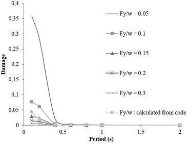
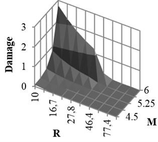
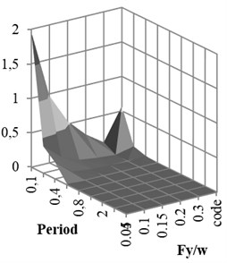
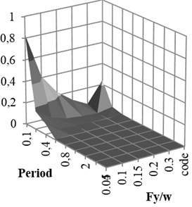
Coefficients of damage attenuation relation of X-braced steel structures for rock and soil conditions are presented in appendix (Tables 6 and 7). In these tables, 162 attenuation relations are presented, which are related to the states listed in Tables 5. The coefficients are constant parameters in Eq. (6) and are obtained through nonlinear regression analysis. In these tables, is standard deviation and is correlation coefficient, obtained from the results of main data regression. Relations 1-27 in Table 5 are related to the mode . This mode is related to the buildings with low strengths. Therefore, the damage of such buildings is expected to be higher than that of other modes. Relations 28-54, 55-81, 82-108, and 109-135 are related to the ratios, respectively, and 136-162 to the () ratio derived from Iranian Earthquake Standard. The correlation coefficient of the results of regression and real data is mostly over 0.92. The damage curve related to the () ratio, obtained from Code is presented in Fig. 6. This curve shows the damage obtained from the attenuation relation model, developed for braced steel structures. According to the figure, the damage decreased with increasing the distance and increased with increasing the magnitude. This result was expected since the beginning owing to the direct relation between ground acceleration and building damage. Moreover, the damage of structures with different periods increased as the ductility capacity decreased. The damage decreased as the strength of structure, that is () ratio, increased (Fig. 7). Therefore, two parameters of () ratio and ductility capacity had direct effects on the damage of buildings. By the way, the structures with low periods and ordinary ductility capacity experienced very strong destructions. This result held true for the buildings with () ratios of higher than 0.2 as well. Accordingly, it is not recommended to construct buildings with ordinary ductility. Fig. 8 shows the curves related to the rock and soil conditions for two () ratios. According to the figure, damage level of the buildings with soil condition was higher than those with rock bed, particularly in lower periods.
Fig. 6Damage curve for Fy/w that calculated from Iranian Code and 0.4 sec period
a) Ordinary ductile
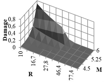
b) Intermediate ductile
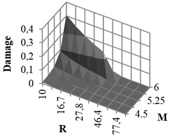
c) Special ductile
6. Verifying nonlinear regression function using neural network method
Neural networks can be considered an alternative approach for modeling process behavior, since they do not need previous knowledge of process phenomenon and only learn by extracting pre-existing patterns from the data which explain the relationship between inputs and outputs in a certain process phenomenon. If appropriate inputs are given to the network, it will acquire knowledge from the environment during a process known as learning. Consequently, the network will assimilate the information that can be recalled later. Neural networks are available in a variety of types, each of which has their distinct architectural differences and reasons for application [16, 21]. Type of neural network used in this work is known as a feed forward network (Fig. 9) and has been found effective in many applications.
There are several different approaches for neural network training, the process of determining an appropriate set of weights, that we used BFGS quasi-Newton method; that is a network training function that updates weight and bias values according to the BFGS quasi-Newton method.
In this study, attempts were made to obtain the relation between damage of X-braced structures, magnitude, and distance. For this purpose, the information of several different earthquake records was gathered from different stations and magnitude and distance were considered as the input parameters of the network; so, the damage related to this record was considered as the output parameter.
Fig. 7Damage curve for different Fy/w and periods
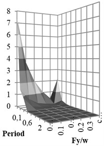
a) Ordinary ductile
b) Intermediate ductile
c) Special ductile
Fig. 8Damage curve for soil and rock conditions M= 5.5, R= 50
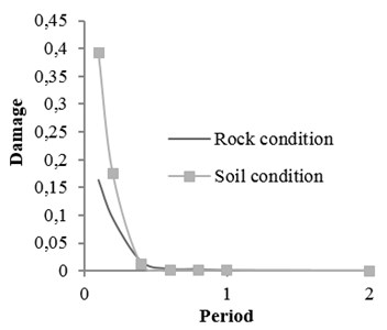
a) calculated from Iranian Code and intermediate ductile
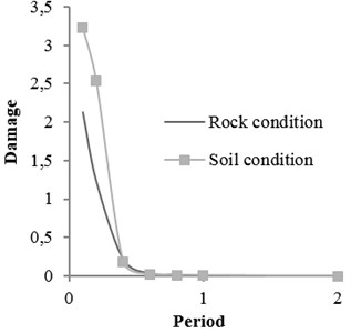
b)0.05 and ordinary ductile
The best result of transfer function was obtained through trial and error method. In this regard, tangent sigmoid was used for the hidden layer, as shown in Eq. (9) and Fig. 10:
Fig. 9Neural network architecture
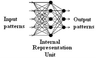
Fig. 10Tansig function shape
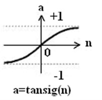
Fig. 11Comparing the real and simulated data for rock condition
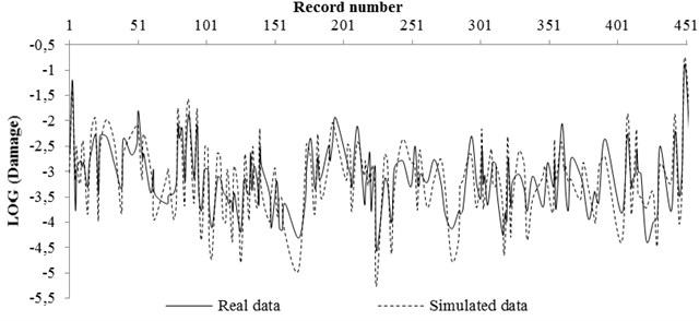
a) NN trained result by 80 % of total data
b) NN tested result by 20 % of total data
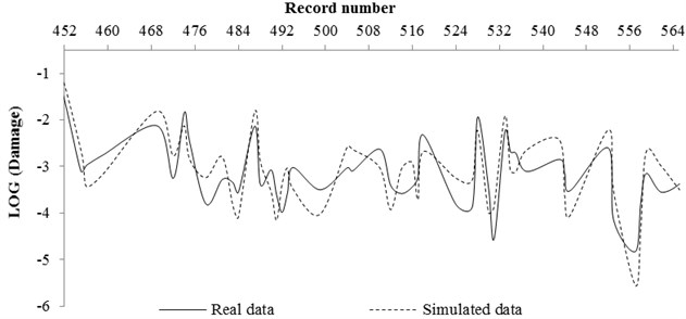
A code was also prepared in Matlab software in order to use neural network. The real data and data simulated by neural network for rock and soil site conditions were compared and shown in Figs. 11 and 12, respectively. The real data were the pattern obtained from Section 4 (stricture damages caused of any record by its magnitude and distance property) and the simulated data were the damage obtained from network prediction. In this work, at first, 80 % of input (magnitude and distance of records) and output (structure damage) pattern data were used for network training and compared by network result. Then, 20 % of input pattern data were used for testing the network and the network result was compared with the real data.
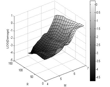
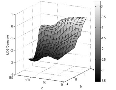
The 3D shape damage attenuation relation was obtained from neural network for X-braced steel structures. It was applied for intermediate ductility and ratio, obtained from Iranian Code and period 1 sec., and shown for rock and soil conditions in Fig. 13.
Since the main objective of this project was to achieve a suitable function to predict structural damage and the neural network was used as a method for verifying the predicted function, in order to evaluate the predicted function obtained in Section 5, the predicted results were compared with those of neural network predictions. Therefore, the standard deviation of prediction errors obtained from the two methods was compared with each other. In other words, as different function forms can be chosen for damage attenuation relation, its certainty was confirmed only through testing other methods. In this section, the results of structural damage prediction obtained from neural network method are compared with those of nonlinear regression (Eq. (7)), shown in Fig. 14.
Fig. 12Comparing the real and simulated data for soil condition
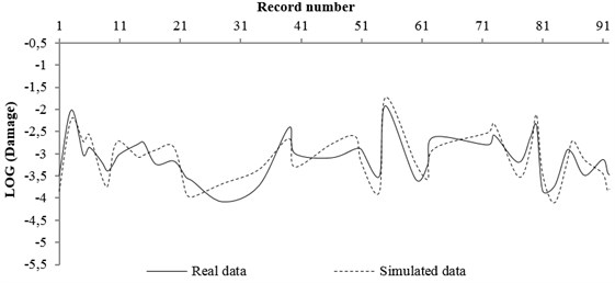
a) NN trained result by 80 % of total data
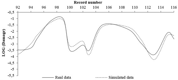
b) NN tested result by 20 % of total data
Fig. 13Rock and soil conditions
a)
b)
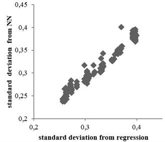
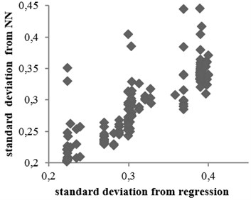
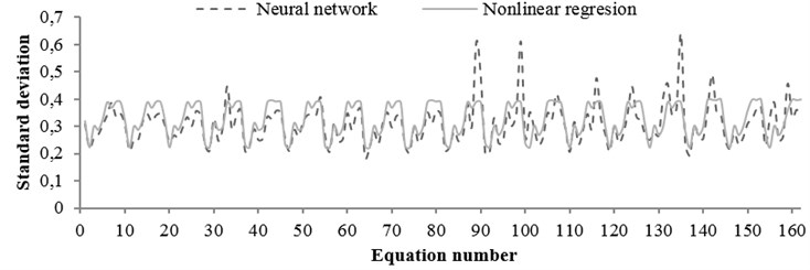
The standard deviation values obtained from the two mentioned methods through all equations for rock and soil conditions are shown in Figs. 15 and 16, respectively. According to the figures, no significant difference was observed between the results. Moreover, in some equations, results of nonlinear regression method had better accuracies. Correlation coefficients between two methods obtained for rock and soil conditions were 0.95 and 0.74, respectively.
As the neural network method is fairly accurately method to predict the data so comparison of the results of neural network and predicted function is thus selected function is suitable for estimating the structural damage.
Fig. 14Standard deviation values obtained from neural network method versus nonlinear regression relation: a) rock condition, b) soil condition
a)
b)
Fig. 15The standard deviation values obtained from regression and neural network for any equation (rock condition)
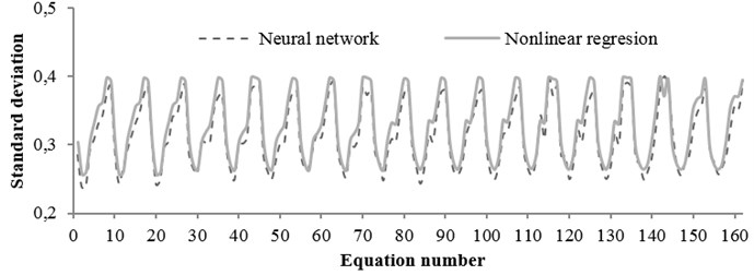
Fig. 16The standard deviation values obtained from regression and neural network for any equation (soil condition)
7. Comparing damage results of time history analysis and attenuation relation
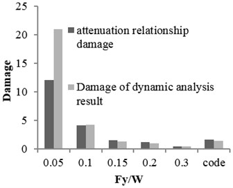
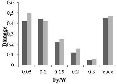
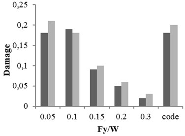
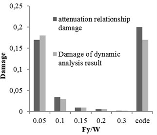
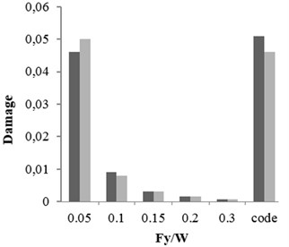
Three buildings with different structural specifications were considered for evaluating the results of attenuation relation, developed for estimating the damage of X-braced steel structures. Nonlinear time history analysis was conducted using Temban record for different () ratios (0.1, 0.15, 0.2, and 0.3) obtained from the Standard (Iranian Code) and different ductility capacities (ordinary, intermediate, and special). The nonlinear specifications of materials were similar to those of one degree of freedom structure, used in the damage spectral design. These buildings were modeled by OpenSees software and their damage values were calculated using the analysis results and Krawinkler damage function. The damage values were calculated by the attenuation relation developed in this research. The parameters, distance () and magnitude () of Temban record, were used to calculate the damage through attenuation relation. The results obtained from two methods were compared and presented in Tables 2-5 and Figs. 17-20. According to the comparison, the results obtained for damage from the developed attenuation relation were acceptably close to those of time history analysis method. The maximum and minimum differences between the results were 40 % and 5 %, respectively. The higher the period of structure, the lower the obtained damage difference. The difference was also higher in the damage values of more than 1. As the damage values of over 1 showed the general destruction of the structure, this difference was of less importance.
Fig. 17The damages obtained from time history analysis and attenuation relation for 2-story building
a) Ordinary ductile
b) Intermediate ductile
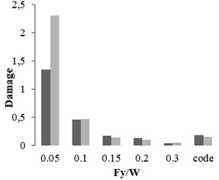
c) Special ductile
Table 2The damages obtained from time history analysis and attenuation relation for 2-story building
Damage obtained by time history analysis and Temban earthquake record | |||||||||||
2 story building 0.4 | |||||||||||
0.05 | 0.1 | 0.15 | 0.2 | 0.3 | Code | ||||||
Ductility | Ordinary | 21 | 4.2 | 1.3 | 0.95 | 0.43 | 1.4 | ||||
Intermediate | 5.6 | 1.1 | 0.3 | 0.25 | 0.11 | 0.37 | |||||
Special | 2.3 | 0.47 | 0.14 | 0.1 | 0.05 | 0.15 | |||||
Damage obtained by attenuation relation for Temban earthquake property ( 6.2, 10.8 km) | |||||||||||
0.4 | |||||||||||
0.05 | 0.1 | 0.15 | 0.2 | 0.3 | Code | ||||||
Ductility | Ordinary | 12.1 | 4.1 | 1.5 | 1.19 | 0.38 | 1.6 | ||||
Intermediate | 3.1 | 1.09 | 0.41 | 0.31 | 0.1 | 0.43 | |||||
Special | 1.35 | 0.46 | 0.17 | 0.13 | 0.04 | 0.18 | |||||
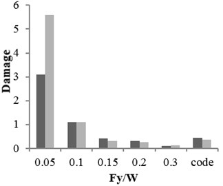
Table 3The damages obtained from time history analysis and attenuation relation for 5-story building
Damage obtained by time history analysis and Temban earthquake record | |||||||||||
5 story building 0.8 | |||||||||||
0.05 | 0.1 | 0.15 | 0.2 | 0.3 | Code | ||||||
Ductility | Ordinary | 1.96 | 1.6 | 0.96 | 0.6 | 0.24 | 1.8 | ||||
Intermediate | 0.5 | 0.42 | 0.25 | 0.16 | 0.06 | 0.47 | |||||
Special | 0.21 | 0.18 | 0.1 | 0.06 | 0.03 | 0.2 | |||||
Damage obtained by attenuation relation for Temban earthquake property ( 6.2, 10.8 km) | |||||||||||
0.4 | |||||||||||
0.05 | 0.1 | 0.15 | 0.2 | 0.3 | Code | ||||||
Ductility | Ordinary | 1.6 | 1.7 | 0.84 | 0.47 | 0.18 | 1.72 | ||||
Intermediate | 0.42 | 0.44 | 0.22 | 0.12 | 0.05 | 0.45 | |||||
Special | 0.18 | 0.19 | 0.09 | 0.05 | 0.02 | 0.18 | |||||
Table 4The damages obtained from time history analysis and attenuation relation for 10-story building
Damage obtained by time history analysis and Temban earthquake record | |||||||||
10 story building 2 | |||||||||
0.05 | 0.1 | 0.15 | 0.2 | 0.3 | Code | ||||
Ductility | Ordinary | 0.18 | 0.03 | 0.01 | 0.006 | 0.0024 | 0.17 | ||
Intermediate | 0.05 | 0.008 | 0.003 | 0.0016 | 0.0006 | 0.046 | |||
Special | 0.02 | 0.003 | 0.0014 | 0.0007 | 0.0002 | 0.019 | |||
Damage obtained by attenuation relation for Temban earthquake property ( 6.2, 10.8 km) | |||||||||
2 | |||||||||
0.05 | 0.1 | 0.15 | 0.2 | 0.3 | Code | ||||
Ductility | Ordinary | 0.17 | 0.034 | 0.008 | 0.0064 | 0.0022 | 0.2 | ||
Intermediate | 0.046 | 0.009 | 0.0025 | 0.0015 | 0.00052 | 0.051 | |||
Special | 0.018 | 0.004 | 0.0012 | 0.00062 | 0.00027 | 0.02 | |||
Fig. 18The damages obtained from time history analysis and attenuation relation for 5-story building
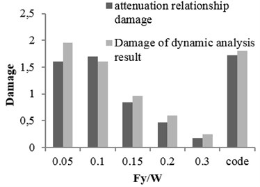
a) Ordinary ductile
b) Intermediate ductile
c) Special ductile
Fig. 19The damages obtained from time history analysis and attenuation relation for 10-story building
a) Ordinary ductile
b) Intermediate ductile
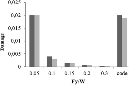
c) Special ductile
8. Probabilistic seismic hazard analysis of damage in Qazvin province using the obtained attenuation relation
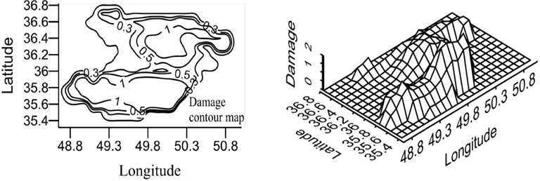
Qazvin province is one of the most seismic regions in Iran and, due to its active faults, it has experienced strong earthquakes in its history. Buinzahra and Roudbar-Manjil earthquakes, the most important events of Iran, happened in this region. In this section, the damage hazard maps of the braced steel structures are prepared using the attenuation relation developed in this research Eq. (6), which was obtained from nonlinear regression and virificated by neural network method as well as probabilistic seismic hazard analysis (PSHA). In this regard, the region was gridded and the hazard damage was obtained by CRISIS software [22] for the earthquake with the returning period of 475 years. The hazard damage maps were plotted for two periods (0.4 and 0.8 sec.) and three ductility levels (ordinary, intermediate, and special), shown in Figs. 20 and 21. In order to use these maps, first, ductility level and period of a building should be defined and then, by having the geographical latitude and longitude of the region, the relevant map can be referred to and the probabilistic damage value under the earthquake with the returning period of 475 years can be found.
It should be mentioned that these maps can be plotted for all periods, soil conditions, and () ratios. However, here, the maps were presented only for the periods 0.4 and 0.8 sec. These maps were related to the buildings cited on the rock bed, the () ratio of which was obtained according to Iranian Code.
According to the maps, the damage level was higher in the south and north areas of Qazvin province compared to its central parts due to the distribution of the active faults of the region. As shown in the damage spectra, the damage level was reduced with the increase in the period. In the constant period, the damage level was reduced as ductility increased. Distribution of damage was the same in different periods because of using the same records in calculating the attenuation relation.
Fig. 20Damage map for X-braced structure, designed by Iranian Code, 0.4 sec. period
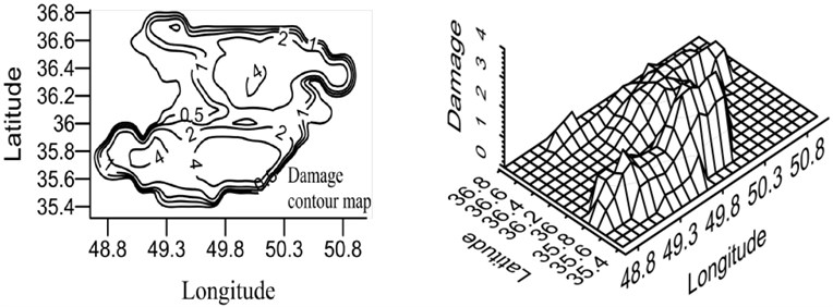
a) Ordinary ductility
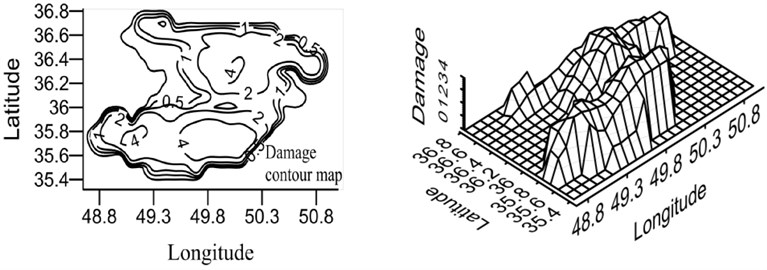
b) Intermediate ductility
c) Special ductility
9. Conclusions
Structural damage can be estimated without conducting time history analysis and preparing damage zoning maps and by having an appropriate attenuation relation with respect to the earthquake magnitude and distance between the site and epicenter. As the risk management centers need rapid and wide evaluation of damage before and after earthquakes, it is crucial to obtain rapid methods for estimating damage and preparing zoning maps.
In this research, the attenuation relation was developed for X-braced steel structures considering the methods of developing acceleration attenuation relation as well as the concept of damage index. For this purpose, after gathering and modifying 772 records, the damage spectrum was prepared using Krawinkler damage function with respect to the logic of acceleration spectrum. Then, a proper function was selected through trial and error process for developing the damage attenuation relation to study the forms of functions used in the acceleration attenuation relations of previous studies. Finally, the coefficients of attenuation relation were obtained by nonlinear regression analysis and neural network method. The results obtained by these two procedures were close to each other.
Fig. 21Damage map for X-braced structure, designed by Iranian Code, 0.8 sec. period

a) Ordinary ductility

b) Intermediate ductility
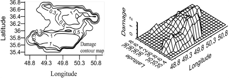
c) Special ductility
In this research, X-braced steel structures were studied for 6 () ratios, 3 levels of ductility, and 9 different periods. 162 groups of coefficients were developed for damage attenuation relation and presented for different nonlinear parameters. The attenuation relation was also developed for soil and rock conditions. In order to compare the damage values obtained from the mentioned relations, time analysis was conducted on 54 structures with different nonlinear specifications and the same records. Then, the damage index was obtained using the analysis results and Krawinkler damage index and compared with the results of developed attenuation relations. The acceptable similarities between these indexes showed the efficiency of attenuation relations developed for calculating the damage of X-braced steel structures.
Having the relations gained in this research, probabilistic risk analysis can be also conducted for damage. The damage zoning was prepared for X-braced structures with different nonlinear parameters in certain regions with respect to the logic of preparing acceleration zoning and probabilistic risk acceleration. The damage zoning maps were prepared for the structures in Qazvin province.
By the way, the attenuation relation, developed in this study, the maps can be similarly prepared for other regions as well. These maps can be directly applied for estimating damage without conducting time history analysis.
References
-
Douglas J. A comprehensive worldwide summary of strong-motion attenuation relationships for peak ground acceleration and spectral ordinates (1969 to 2000). Engineering Seismology and Earthquake Engineering, 2001.
-
Battis J. Regional modification of acceleratior attenuation functions. Bulletin of the Seismological Society of America, Vol. 71, Issue 4, 1981, p. 1309-1321.
-
Campbell K. W. Near-source attenuation of peak horizontal acceleration. Bulletin of the Seismological Society of America, Vol. 71, Issue 6, 1981, p. 2039-2070.
-
Joyner W. B., Boore D. M. Peak horizontal acceleration and velocity from strong-motion records including records from the 1979 imperial valley California earthquake. Bulletin of the Seismological Society of America, Vol. 71, Issue 6, 1981, p. 2011-2038.
-
Boore D. M., JoynerW. B. The empirical prediction of ground motion. Bulletin of the Seismological Society of American, Vol. 72, Issue 6, 1982, p. S43-S60.
-
Joyner W. B., Boore D. M. Measurement, characterization, and prediction of strong ground motion, Proceedings of Earthquake Engineering and Soil Dynamics II, Geotechnical Division, 1988, p. 43-102.
-
Atkinson G. M., Boore D. M. Recent trends in ground motion and spectral response relations for North America. Earthquake Spectra, Vol. 6, Issue 1, p. 1990, p. 15-35.
-
Douglas J. Earthquake ground motion estimation using strong motion records: A review of equations for estimation of peak ground acceleration and response ordinates. Earth-Science Reviews, Vol. 61, Issue 1-2, 2003, p. 43-104.
-
Bragato P. L., Slejko D. Empirical ground-motion attenuation relations for the Eastern Alps in the magnitude range 2.5-6.3. Bulletin of the Seismological Society of American, Vol. 95, Issue 1, 2005, p. 252-276.
-
Ghodrati Amiri G., Mahdavian A., Manouchehri Dana F. Attenuation relationshipship for Iran. Journal of Earthquake Engineering, Vol. 11, Issue 4, 2007, p. 469-492.
-
Bragato P. L. Assessing regional and site-dependent variability of ground motions for ShakeMap implementation in Italy. Bulletin of the Seismological Society of America, Vol. 99, Issue 5, 2009, p. 2950-2960.
-
Pacific Earthquake Engineering Research Center. NGA-West2 research Project http://daveboore.com/pubs_online/Bozorgnia_et_al_NGA_West2_overview_EQS_Dec8_2013_clean.pdf, 2013.
-
Bozorgnia Y., Bertero V. Damage spectra: characteristics and applications to seismic risk reduction. Journal of Structural Engineering, Vol. 129, Issue 10, 2003, p. 1330-1340.
-
Krawinkler H., Zohrei M. Cumulative damage in steel structures subjected to earthquake ground motions. Computers and Structures, Vol. 16, 1983, p. 531-541.
-
Mazzoni S., McKenna F.,Scott M. H., Fenves G. L., et al. OpenSees Command Language Manual, 2007.
-
Demuth H., Beale M., Hagan M. Neural Network Toolbox for use with MATLAB. The Mathworks, 2006.
-
Permanent Committee for Revising the Iranian Code of Practice for Seismic Resistant Design of Buildings. Standard2800: 2nd Edition, Iranian code of practice for seismic resistance design of buildings, Tehran, Iran, 1999.
-
Campbell K. W., Bozorgnia Y. Campbell–Bozorgnia NGA empirical ground motion model for the average horizontal component of PGA, PGV, PGD and SA at selected spectral periods ranging from 0.01-10.0 seconds (Oct. 16). University of California, Berkeley, Pacifc Earthquake Engineering Research Center, PEER-Lifelines Next Generation Attenuation of Ground Motion (NGA) Project, 2006.
-
Iranian Committee of Large Dams. IRCOLD: Relationshipship between Ms and Mb. Tehran, Iran, 1994.
-
Matlab (7.6.0.324 (R2008a)). The Language of Technical Computing. USA, Math Works, Inc, U.S. patents.
-
Haykin S. Neural Networks: A Comprehensive Foundation. Prentice Hall, 1999.
-
CRISIS2007 (7.6). Program for computing seismic hazard. Mexico, Derechos Reservados.
-
Opensees (2.4). Open system for earthquake engineering simulation. University of California, Berkeley, Pacifc Earthquake Engineering Research Center.
About this article

